Triangle#
Introduction#
With this User Guide, we will be covering all of the core functionality of chainladder.
All important user functionality can be referenced from the top level of the library and
so importing the library as the cl namespace is the preferred way of importing from chainladder.
import chainladder as cl

import matplotlib.pyplot as plt
plt.style.use('ggplot')
%config InlineBackend.figure_format = 'retina'
Analysis is the intersection of data, models, and assumptions.
Reserving analysis is no different and the loss Triangle is the most ubiquitous data construct used by actuaries today. The chainladder package has its own :class:Triangle data structure that behaves much like a pandas DataFrame.
Why not Pandas?#
This begs the question, why not just use pandas? There are several advantages over having a dedicated Triangle object:
Actuaries work with sets of triangles. DataFrames, being two dimensional, support single triangles with grace but become unwieldy with multiple triangles.
We can carry through the meaningful pandas functionality while also supporting triangle specific methods not found in pandas
Improved memory footprint with sparse array representation in backend
Calculated fields with “virtual” columns allows for lazy column evaluation of Triangles as well as improved memory footprint for larger triangles.
Ability to support GPU-based backends.
Ultimately, there are a lot of things pandas can do that are not relevant to reserving, and there are a lot of things a Triangle needs to do that are not handled easily with pandas.
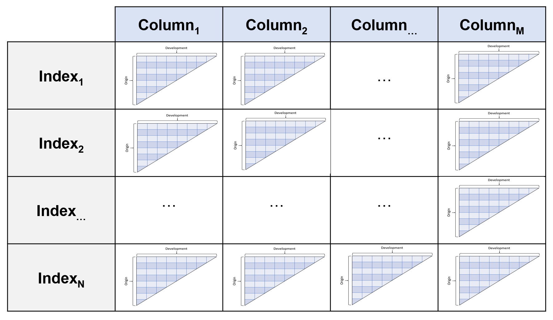
Structure#
The :class:Triangle is the data structure of the chainladder package. Just as
Scikit-learn likes to only consume numpy arrays, Chainladder only likes
Triangles. It is a 4D data structure with labeled axes. These axes are its
index, columns, origin, development.
index (axis 0):
The index is the lowest grain at which you want to manage the triangle.
These can be things like state or company. Like a pandas.multiIndex, you
can throw more than one column into the index.
columns (axis 1):
Columns are where you would want to store the different numeric values of your
data. Paid, Incurred, Counts are all reasonable choices for the columns of your
triangle.
origin (axis 2):
The origin is the period of time from which your columns originate. It can
be an Accident Month, Report Year, Policy Quarter or any other period-like vector.
development (axis 3):
Development represents the development age or date of your triangle.
Valuation Month, Valuation Year, Valuation Quarter are good choices.
Despite this structure, you interact with it in the style of pandas. You would
use index and columns in the same way you would for a pandas DataFrame.
You can think of the 4D structure as a pandas DataFrame where each cell (row,
column) is its own triangle.
Like pandas, you can access the values property of a triangle to get its numpy
representation, however the Triangle class provides many helper methods to
keep the shape of the numpy representation in sync with the other Triangle
properties.
Creating a Triangle#
Basic requirements#
You must have a pandas DataFrame on hand to create a triangle. While data can come in a variety of forms those formats should be coerced to a pandas DataFrame before creating a triangle. The DataFrame also must be in tabular (long) format, not triangle (wide) format:
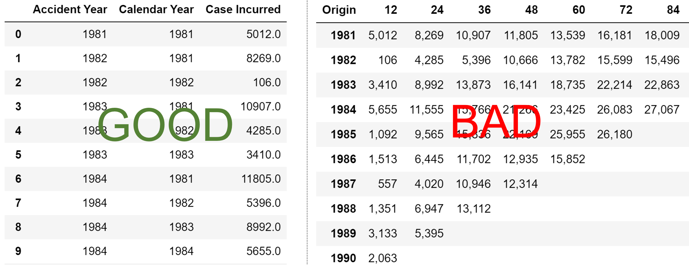
At a minimum, the DataFrame must also:
have “date-like” columns for the
originanddevelopmentperiod of the triangle.Have a numeric column(s) representing the amount(s) of the triangle.
The reason for these restriction is that the :class:Triangle infers a lot of
useful properties from your DataFrame. For example, it will determine the grain
and valuation_date of your triangle which in turn are used to derive many
other properties of your triangle without further prompting from you.
Date Inference#
When instantiating a :class:Triangle, the origin and development
arguments can take a str representing the column name in your pandas DataFrame
that contains the relevant information. Alternatively, the arguments can also
take a list in the case where your DataFrame includes multiple columns that
represent the dimension, e.g. ['accident_year','accident_quarter'] can be
supplied to create an origin dimension at the accident quarter grain.
cl.Triangle(data, origin='Acc Year', development=['Cal Year', 'Cal Month'], columns=['Paid Loss'])
The :class:Triangle relies heavily on pandas date inference. In fact,
pd.to_datetime(date_like) is exactly how it works. While pandas is excellent
at inference, it is not perfect. When initializing a Triangle you can always
use the origin_format and/or development_format arguments to force
the inference. For example, origin_format='%Y/%m/%d'
Multidimensional Triangle#
So far we’ve seen how to create a single Triangle, but as described in the Intro
the Triangle class can hold multiple triangles at once. These triangles share the
same origin and development axes and act as individual cells would in a
pandas DataFrame. By specifying one or more column and one or more index,
we can fill out the 4D triangle structure.
cl.Triangle(data, origin='Acc Year', development='Cal Year',
            columns=['Paid Loss', 'Incurred Loss'],
            index=['Line of Business', 'State'])
Sample Data#
The chainladder package has several sample triangles. Many of these come
from existing papers and can be used to verify the results of those papers.
Additionally, They are a quick way of exploring the functionality of the package.
These triangles can be called by name using the :func:~chainladder.load_sample function.
cl.load_sample('clrd')
| Triangle Summary | |
|---|---|
| Valuation: | 1997-12 |
| Grain: | OYDY |
| Shape: | (775, 6, 10, 10) |
| Index: | [GRNAME, LOB] |
| Columns: | [IncurLoss, CumPaidLoss, BulkLoss, EarnedPremDIR, EarnedPremCeded, EarnedPremNet] |
Other Parameters#
Whether a triangle is cumulative or incremental in nature cannot be inferred
from the “date-like” vectors of your DataFrame. You can optionally specify this
property with the cumulative parameter.
cl.Triangle(
    data, origin='Acc Year', development=['Cal Year'],
    columns=['PaidLoss'], cumulative=True)
Note
The cumulative parameter is completely optional. If it is not specified,
the Triangle will infer its cumulative/incremental status at the point you
call on the cum_to_incr or incr_to_cum methods discussed below. Some methods
may not work until the cumulative/incremental status is known.
Backends
Triangle is built on numpy which serves as the array backend by default.
However, you can now swap array_backend between numpy, cupy, and sparse to switch
between CPU and GPU-based computations or dense and sparse backends.
Array backends can be set globally:
cl.options.set_option('array_backend', 'cupy')
cl.options.reset_option()
Alternatively, they can be set per Triangle instance.
cl.Triangle(..., array_backend='cupy')
Note
You must have a CUDA-enabled graphics card and CuPY installed to use the GPU backend. These are optional dependencies of chainladder.
Chainladder by default will swap between the numpy and sparse backends. This
substantially improves the memory footprint of chainladder substantially beyond
what can be achieved with pandas alone. When a Triangle becomes sufficiently large
and has a lot of 0 or null entries, the triangle will silently swap between the
numpy and sparse backends.
prism = cl.load_sample('prism')
prism
/home/docs/checkouts/readthedocs.org/user_builds/chainladder-python/conda/latest/lib/python3.11/site-packages/chainladder/core/base.py:250: UserWarning: The argument 'infer_datetime_format' is deprecated and will be removed in a future version. A strict version of it is now the default, see https://pandas.pydata.org/pdeps/0004-consistent-to-datetime-parsing.html. You can safely remove this argument.
  arr = dict(zip(datetime_arg, pd.to_datetime(**item)))
| Triangle Summary | |
|---|---|
| Valuation: | 2017-12 |
| Grain: | OMDM |
| Shape: | (34244, 4, 120, 120) |
| Index: | [ClaimNo, Line, Type, ClaimLiability, Limit, Deductible] |
| Columns: | [reportedCount, closedPaidCount, Paid, Incurred] |
prism.array_backend
'sparse'
prism.sum().array_backend
'numpy'
You can globally disable the backend swapping by invoking auto_sparse(False).
Any triangle with a cupy backend will not invoke auto_sparse. In the future it may be supported
when there is better sparse-GPU array support.:
cl.options.set_option('auto_sparse', False)
prism = cl.load_sample('prism', array_backend='sparse')
prism.array_backend
/home/docs/checkouts/readthedocs.org/user_builds/chainladder-python/conda/latest/lib/python3.11/site-packages/chainladder/core/base.py:250: UserWarning: The argument 'infer_datetime_format' is deprecated and will be removed in a future version. A strict version of it is now the default, see https://pandas.pydata.org/pdeps/0004-consistent-to-datetime-parsing.html. You can safely remove this argument.
  arr = dict(zip(datetime_arg, pd.to_datetime(**item)))
'sparse'
prism.sum().array_backend
'numpy'
Warning
Loading ‘prism’ with the numpy backend will consume all of your systems memory.
Basic Functionality#
Representation#
The Triangle has two different representations. When only a single
index AND single column is selected. The triangle is the typical 2-dimensional
representation we typically think of.
triangle = cl.load_sample('ukmotor')
print(triangle.shape)
triangle
(1, 1, 7, 7)
| 12 | 24 | 36 | 48 | 60 | 72 | 84 | |
|---|---|---|---|---|---|---|---|
| 2007 | 3,511 | 6,726 | 8,992 | 10,704 | 11,763 | 12,350 | 12,690 |
| 2008 | 4,001 | 7,703 | 9,981 | 11,161 | 12,117 | 12,746 | |
| 2009 | 4,355 | 8,287 | 10,233 | 11,755 | 12,993 | ||
| 2010 | 4,295 | 7,750 | 9,773 | 11,093 | |||
| 2011 | 4,150 | 7,897 | 10,217 | ||||
| 2012 | 5,102 | 9,650 | |||||
| 2013 | 6,283 |
If more than one index or more than one column is present, then the Triangle
takes on more of a summary view.
triangle = cl.load_sample('CLRD')
print(triangle.shape)
triangle
(775, 6, 10, 10)
| Triangle Summary | |
|---|---|
| Valuation: | 1997-12 |
| Grain: | OYDY |
| Shape: | (775, 6, 10, 10) |
| Index: | [GRNAME, LOB] |
| Columns: | [IncurLoss, CumPaidLoss, BulkLoss, EarnedPremDIR, EarnedPremCeded, EarnedPremNet] |
Valuation vs Development#
While most Estimators that use triangles expect the development period to be
expressed as an origin age, it is possible to transform a triangle into a valuation
triangle where the development periods are converted to valuation periods. Expressing
triangles this way may provide a more convenient view of valuation slices.
Switching between a development triangle and a valuation triangle can be
accomplished with the method dev_to_val and its inverse val_to_dev.
cl.load_sample('raa').dev_to_val()
| 1981 | 1982 | 1983 | 1984 | 1985 | 1986 | 1987 | 1988 | 1989 | 1990 | |
|---|---|---|---|---|---|---|---|---|---|---|
| 1981 | 5,012 | 8,269 | 10,907 | 11,805 | 13,539 | 16,181 | 18,009 | 18,608 | 18,662 | 18,834 |
| 1982 | 106 | 4,285 | 5,396 | 10,666 | 13,782 | 15,599 | 15,496 | 16,169 | 16,704 | |
| 1983 | 3,410 | 8,992 | 13,873 | 16,141 | 18,735 | 22,214 | 22,863 | 23,466 | ||
| 1984 | 5,655 | 11,555 | 15,766 | 21,266 | 23,425 | 26,083 | 27,067 | |||
| 1985 | 1,092 | 9,565 | 15,836 | 22,169 | 25,955 | 26,180 | ||||
| 1986 | 1,513 | 6,445 | 11,702 | 12,935 | 15,852 | |||||
| 1987 | 557 | 4,020 | 10,946 | 12,314 | ||||||
| 1988 | 1,351 | 6,947 | 13,112 | |||||||
| 1989 | 3,133 | 5,395 | ||||||||
| 1990 | 2,063 |
Triangles have the is_val_tri property that denotes whether a triangle is in valuation
mode. The latest diagonal of a Triangle is a valuation triangle.
cl.load_sample('raa').latest_diagonal.is_val_tri
True
Incremental vs Cumulative#
A triangle is either cumulative or incremental. The is_cumulative
property will identify this trait. Accumulating an incremental triangle can
be acomplished with incr_to_cum. The inverse operation is cum_to_incr.
raa = cl.load_sample('raa')
print(raa.is_cumulative)
raa.cum_to_incr()
True
| 12 | 24 | 36 | 48 | 60 | 72 | 84 | 96 | 108 | 120 | |
|---|---|---|---|---|---|---|---|---|---|---|
| 1981 | 5,012 | 3,257 | 2,638 | 898 | 1,734 | 2,642 | 1,828 | 599 | 54 | 172 |
| 1982 | 106 | 4,179 | 1,111 | 5,270 | 3,116 | 1,817 | -103 | 673 | 535 | |
| 1983 | 3,410 | 5,582 | 4,881 | 2,268 | 2,594 | 3,479 | 649 | 603 | ||
| 1984 | 5,655 | 5,900 | 4,211 | 5,500 | 2,159 | 2,658 | 984 | |||
| 1985 | 1,092 | 8,473 | 6,271 | 6,333 | 3,786 | 225 | ||||
| 1986 | 1,513 | 4,932 | 5,257 | 1,233 | 2,917 | |||||
| 1987 | 557 | 3,463 | 6,926 | 1,368 | ||||||
| 1988 | 1,351 | 5,596 | 6,165 | |||||||
| 1989 | 3,133 | 2,262 | ||||||||
| 1990 | 2,063 |
Triangle Grain#
If your triangle has origin and development grains that are more frequent then
yearly, you can easily swap to a higher grain using the grain method of the
Triangle. The grain method recognizes Yearly (Y), Quarterly (Q), and
Monthly (M) grains for both the origin period and development period.
cl.load_sample('quarterly')
/home/docs/checkouts/readthedocs.org/user_builds/chainladder-python/conda/latest/lib/python3.11/site-packages/chainladder/core/base.py:250: UserWarning: The argument 'infer_datetime_format' is deprecated and will be removed in a future version. A strict version of it is now the default, see https://pandas.pydata.org/pdeps/0004-consistent-to-datetime-parsing.html. You can safely remove this argument.
  arr = dict(zip(datetime_arg, pd.to_datetime(**item)))
/home/docs/checkouts/readthedocs.org/user_builds/chainladder-python/conda/latest/lib/python3.11/site-packages/chainladder/core/base.py:250: UserWarning: Could not infer format, so each element will be parsed individually, falling back to `dateutil`. To ensure parsing is consistent and as-expected, please specify a format.
  arr = dict(zip(datetime_arg, pd.to_datetime(**item)))
| Triangle Summary | |
|---|---|
| Valuation: | 2006-03 |
| Grain: | OYDQ |
| Shape: | (1, 2, 12, 45) |
| Index: | [Total] |
| Columns: | [incurred, paid] |
cl.load_sample('quarterly').grain('OYDY')
/home/docs/checkouts/readthedocs.org/user_builds/chainladder-python/conda/latest/lib/python3.11/site-packages/chainladder/core/base.py:250: UserWarning: The argument 'infer_datetime_format' is deprecated and will be removed in a future version. A strict version of it is now the default, see https://pandas.pydata.org/pdeps/0004-consistent-to-datetime-parsing.html. You can safely remove this argument.
  arr = dict(zip(datetime_arg, pd.to_datetime(**item)))
/home/docs/checkouts/readthedocs.org/user_builds/chainladder-python/conda/latest/lib/python3.11/site-packages/chainladder/core/base.py:250: UserWarning: Could not infer format, so each element will be parsed individually, falling back to `dateutil`. To ensure parsing is consistent and as-expected, please specify a format.
  arr = dict(zip(datetime_arg, pd.to_datetime(**item)))
| Triangle Summary | |
|---|---|
| Valuation: | 2006-03 |
| Grain: | OYDY |
| Shape: | (1, 2, 12, 12) |
| Index: | [Total] |
| Columns: | [incurred, paid] |
It is generally a good practice to bring your data in at the lowest grain available, so that you have full flexibility in aggregating to the grain of your choosing for analysis and separately, the grain of your choosing for reporting and communication.
Link Ratios#
The age-to-age factors or link ratios of a Triangle can be accessed with the
link_ratio property. Triangles also have a heatmap method that can optionally
be called to apply conditional formatting to triangle values along an axis. The
heatmap method requires IPython/Jupyter notebook to render.
triangle = cl.load_sample('abc')
triangle.link_ratio.heatmap()
| 12-24 | 24-36 | 36-48 | 48-60 | 60-72 | 72-84 | 84-96 | 96-108 | 108-120 | 120-132 | |
|---|---|---|---|---|---|---|---|---|---|---|
| 1977 | 2.2263 | 1.3933 | 1.1835 | 1.1070 | 1.0679 | 1.0468 | 1.0304 | 1.0231 | 1.0196 | 1.0163 |
| 1978 | 2.2682 | 1.3924 | 1.1857 | 1.1069 | 1.0649 | 1.0451 | 1.0301 | 1.0267 | 1.0207 | |
| 1979 | 2.2331 | 1.4014 | 1.1871 | 1.1068 | 1.0649 | 1.0418 | 1.0352 | 1.0276 | ||
| 1980 | 2.1988 | 1.3944 | 1.2021 | 1.1014 | 1.0702 | 1.0496 | 1.0394 | |||
| 1981 | 2.2115 | 1.4004 | 1.1764 | 1.1094 | 1.0706 | 1.0536 | ||||
| 1982 | 2.2290 | 1.3872 | 1.2037 | 1.1264 | 1.0956 | |||||
| 1983 | 2.2918 | 1.4296 | 1.2197 | 1.1337 | ||||||
| 1984 | 2.3731 | 1.4654 | 1.2283 | |||||||
| 1985 | 2.4457 | 1.4704 | ||||||||
| 1986 | 2.4031 |
The Triangle link_ratio property has unique properties from regular triangles.
They are considered patterns.
triangle.link_ratio.is_pattern
True
They are considered incremental, and accumulate in a multiplicative fashion.
triangle = cl.load_sample('abc')
triangle.link_ratio.incr_to_cum()
| 12-Ult | 24-Ult | 36-Ult | 48-Ult | 60-Ult | 72-Ult | 84-Ult | 96-Ult | 108-Ult | 120-Ult | |
|---|---|---|---|---|---|---|---|---|---|---|
| 1977 | 4.9633 | 2.2293 | 1.6000 | 1.3519 | 1.2213 | 1.1436 | 1.0924 | 1.0601 | 1.0362 | 1.0163 |
| 1978 | 4.9795 | 2.1954 | 1.5767 | 1.3298 | 1.2014 | 1.1282 | 1.0795 | 1.0479 | 1.0207 | |
| 1979 | 4.8528 | 2.1731 | 1.5507 | 1.3063 | 1.1802 | 1.1083 | 1.0638 | 1.0276 | ||
| 1980 | 4.7394 | 2.1555 | 1.5458 | 1.2859 | 1.1675 | 1.0910 | 1.0394 | |||
| 1981 | 4.5594 | 2.0616 | 1.4722 | 1.2514 | 1.1280 | 1.0536 | ||||
| 1982 | 4.5932 | 2.0607 | 1.4855 | 1.2341 | 1.0956 | |||||
| 1983 | 4.5302 | 1.9767 | 1.3827 | 1.1337 | ||||||
| 1984 | 4.2715 | 1.8000 | 1.2283 | |||||||
| 1985 | 3.5962 | 1.4704 | ||||||||
| 1986 | 2.4031 |
Commutativity#
Where possible, the triangle methods are designed to be commutative. For example, each of these operations is functionally equivalent.
tri = cl.load_sample('quarterly')
# Functionally equivalent transformations
tri.grain('OYDY').val_to_dev() == tri.val_to_dev().grain('OYDY')
tri.cum_to_incr().grain('OYDY').val_to_dev() == tri.val_to_dev().cum_to_incr().grain('OYDY')
tri.grain('OYDY').cum_to_incr().val_to_dev().incr_to_cum() == tri.val_to_dev().grain('OYDY')
/home/docs/checkouts/readthedocs.org/user_builds/chainladder-python/conda/latest/lib/python3.11/site-packages/chainladder/core/base.py:250: UserWarning: The argument 'infer_datetime_format' is deprecated and will be removed in a future version. A strict version of it is now the default, see https://pandas.pydata.org/pdeps/0004-consistent-to-datetime-parsing.html. You can safely remove this argument.
  arr = dict(zip(datetime_arg, pd.to_datetime(**item)))
/home/docs/checkouts/readthedocs.org/user_builds/chainladder-python/conda/latest/lib/python3.11/site-packages/chainladder/core/base.py:250: UserWarning: Could not infer format, so each element will be parsed individually, falling back to `dateutil`. To ensure parsing is consistent and as-expected, please specify a format.
  arr = dict(zip(datetime_arg, pd.to_datetime(**item)))
True
Performance Tips#
Being mindful of commutativity and computational intensity can really help improve the performance of the package, particularly for really large triangles. Consider these examples that produce identical outputs but with drastically different performance. In general, aggregations reduce the number of cells in a Triangle and should come as early in your method chain as possible.
import timeit
prism = cl.load_sample('prism')
# Accumulation before aggregation - BAD
timeit.timeit(lambda : prism.incr_to_cum().sum(), number=1)
/home/docs/checkouts/readthedocs.org/user_builds/chainladder-python/conda/latest/lib/python3.11/site-packages/chainladder/core/base.py:250: UserWarning: The argument 'infer_datetime_format' is deprecated and will be removed in a future version. A strict version of it is now the default, see https://pandas.pydata.org/pdeps/0004-consistent-to-datetime-parsing.html. You can safely remove this argument.
  arr = dict(zip(datetime_arg, pd.to_datetime(**item)))
10.157972535999988
# Aggregation before accumulation - GOOD
timeit.timeit(lambda : prism.sum().incr_to_cum(), number=1)
0.02395860700016783
In other cases, querying the Triangle in clever ways can improve performance.
Consider that the latest_diagonal of a cumulative Triangle is equal to the
sum of its incremental values along the ‘development’ axis.
# Accumulating a large triangle to get latest_diagonal - BAD
timeit.timeit(lambda : prism.incr_to_cum().latest_diagonal, number=1)
9.175006923999945
# Summing incrementals of a large triangle to get latest_diagonal - GOOD
timeit.timeit(lambda : prism.sum('development'), number=1)
0.03220626000006632
Trend#
A uniform trend factor can also be applied to a Triangle. The trend can
be applied along the origin or valuation axes.
tri = cl.load_sample('ukmotor')
# Dividing by original triangle to show the trend factor
tri.trend(0.05, axis='valuation')/tri
| 12 | 24 | 36 | 48 | 60 | 72 | 84 | |
|---|---|---|---|---|---|---|---|
| 2007 | 1.3401 | 1.2763 | 1.2155 | 1.1576 | 1.1025 | 1.0500 | 1.0000 |
| 2008 | 1.2763 | 1.2155 | 1.1576 | 1.1025 | 1.0500 | 1.0000 | |
| 2009 | 1.2155 | 1.1576 | 1.1025 | 1.0500 | 1.0000 | ||
| 2010 | 1.1576 | 1.1025 | 1.0500 | 1.0000 | |||
| 2011 | 1.1025 | 1.0500 | 1.0000 | ||||
| 2012 | 1.0500 | 1.0000 | |||||
| 2013 | 1.0000 |
While the trend method only allows for a single trend, you can create
compound trends using start and end arguments and chaining them together.
tri.trend(0.05, axis='valuation', start=tri.valuation_date, end='2011-12-31') \
   .trend(0.10, axis='valuation', start='2011-12-31')/tri
| 12 | 24 | 36 | 48 | 60 | 72 | 84 | |
|---|---|---|---|---|---|---|---|
| 2007 | 1.6142 | 1.4674 | 1.3340 | 1.2128 | 1.1025 | 1.0500 | 1.0000 |
| 2008 | 1.4674 | 1.3340 | 1.2128 | 1.1025 | 1.0500 | 1.0000 | |
| 2009 | 1.3340 | 1.2127 | 1.1025 | 1.0500 | 1.0000 | ||
| 2010 | 1.2128 | 1.1025 | 1.0500 | 1.0000 | |||
| 2011 | 1.1025 | 1.0500 | 1.0000 | ||||
| 2012 | 1.0500 | 1.0000 | |||||
| 2013 | 1.0000 |
Correlation Tests#
The multiplicative chainladder method is based on the strong assumptions of independence across origin years and across valuation years. Mack developed tests to verify if these assumptions hold.
These tests are included as methods on the triangle class valuation_correlation
and development_correlation. False indicates that correlation between years
is not sufficiently large.
triangle = cl.load_sample('raa')
triangle.valuation_correlation().z_critical
/home/docs/checkouts/readthedocs.org/user_builds/chainladder-python/conda/latest/lib/python3.11/site-packages/numpy/lib/nanfunctions.py:1217: RuntimeWarning: All-NaN slice encountered
  return function_base._ureduce(a, func=_nanmedian, keepdims=keepdims,
| 1982 | 1983 | 1984 | 1985 | 1986 | 1987 | 1988 | 1989 | 1990 | |
|---|---|---|---|---|---|---|---|---|---|
| 1981 | False | False | False | False | False | False | False | False | False |
triangle.development_correlation().t_critical
There are many properties of these correlation tests and they’ve been included
as their own classes. Refer to ValuationCorrelation and
DevelopmentCorrelation for additional information.
Pandas-style syntax#
We’ve chosen to keep as close as possible to pandas syntax for Triangle data
manipulation. Relying on the most widely used data manipulation library in Python
gives us two benefits. This not only allows for easier adoption, but also provides
stability to the chainladder API.
Slicing and Filtering#
With a newly minted Triangle, individual triangles can be sliced out
of the object using pandas-style loc/iloc or boolean filtering.
clrd = cl.load_sample('clrd')
clrd.iloc[0,1]
clrd[clrd['LOB']=='othliab']
clrd['EarnedPremDIR']
| Triangle Summary | |
|---|---|
| Valuation: | 1997-12 |
| Grain: | OYDY |
| Shape: | (775, 1, 10, 10) |
| Index: | [GRNAME, LOB] |
| Columns: | [EarnedPremDIR] |
Note
Boolean filtering on non-index columns in pandas feels natural. We’ve exposed
the same syntax specifically for the index column(s) of the Triangle without the
need for reset_index() or trying to boolean-filter a MultiIndex. This is
a divergence from the pandas API.
As of version 0.7.6, four-dimensional slicing is supported:
clrd = cl.load_sample('clrd')
clrd.iloc[[0, 10, 3], 1:8, :5, :]
clrd.loc[:'Aegis Grp', 'CumPaidLoss':, '1990':'1994', :48]
| Triangle Summary | |
|---|---|
| Valuation: | 1997-12 |
| Grain: | OYDY |
| Shape: | (5, 5, 5, 4) |
| Index: | [GRNAME, LOB] |
| Columns: | [CumPaidLoss, BulkLoss, EarnedPremDIR, EarnedPremCeded, EarnedPremNet] |
As of version 0.8.3, .iat and at functionality have been added. Similar
to pandas, one can use these for value assignment for a single cell of a Triangle.
When a ‘sparse’ backend is in use, these accessors are the only way to modify individual
cells of a triangle.
raa = cl.load_sample('raa').set_backend('sparse')
# To modify a sparse triangle, we need to use at or iat
raa.at['Total', 'values', '1985', 12] = 10000
Arithmetic#
Most arithmetic operations can be used to create new triangles within your
triangle instance. Like with pandas, these can automatically be added as new
columns to your Triangle.
clrd = cl.load_sample('clrd')
clrd['CaseIncur'] = clrd['IncurLoss']-clrd['BulkLoss']
clrd
| Triangle Summary | |
|---|---|
| Valuation: | 1997-12 |
| Grain: | OYDY |
| Shape: | (775, 7, 10, 10) |
| Index: | [GRNAME, LOB] |
| Columns: | [IncurLoss, CumPaidLoss, BulkLoss, EarnedPremDIR, EarnedPremCeded, EarnedPremNet, CaseIncur] |
For origin and development axes, arithmetic follows numpy broadcasting <https://numpy.org/doc/1.18/user/theory.broadcasting.html#array-broadcasting-in-numpy>_
rules. If broadcasting fails, arithmetic operations will rely on origin and
development vectors to determine whether an operation is legal.
raa = cl.load_sample('raa')
# Allow for arithmetic beyond numpy broadcasting rules
raa[raa.origin<'1985']+raa[raa.origin>='1985']
| 12 | 24 | 36 | 48 | 60 | 72 | 84 | 96 | 108 | 120 | |
|---|---|---|---|---|---|---|---|---|---|---|
| 1981 | 5,012 | 8,269 | 10,907 | 11,805 | 13,539 | 16,181 | 18,009 | 18,608 | 18,662 | 18,834 |
| 1982 | 106 | 4,285 | 5,396 | 10,666 | 13,782 | 15,599 | 15,496 | 16,169 | 16,704 | |
| 1983 | 3,410 | 8,992 | 13,873 | 16,141 | 18,735 | 22,214 | 22,863 | 23,466 | ||
| 1984 | 5,655 | 11,555 | 15,766 | 21,266 | 23,425 | 26,083 | 27,067 | |||
| 1985 | 1,092 | 9,565 | 15,836 | 22,169 | 25,955 | 26,180 | ||||
| 1986 | 1,513 | 6,445 | 11,702 | 12,935 | 15,852 | |||||
| 1987 | 557 | 4,020 | 10,946 | 12,314 | ||||||
| 1988 | 1,351 | 6,947 | 13,112 | |||||||
| 1989 | 3,133 | 5,395 | ||||||||
| 1990 | 2,063 |
# Numpy broadcasting equivalent fails
raa[raa.origin<'1985'].values+raa[raa.origin>='1985'].values
Arithmetic between two Triangles with different labels will align the axes of each Triangle consistent with arithmetic of a pandas Series. Bypassing index matching can be accomplished with arithmetic between an Triangle and an array.
s1 = cl.load_sample('clrd').iloc[:3]
s2 = s1.sort_index(ascending=False)
s1 + s2 == 2 * s1
True
s1 + s2.values == 2 * s1
False
s3 = s1.iloc[:, ::-1]
s1 + s3 == 2 * s1
True
Virtual Columns#
There are instances where we want to defer calculations, we can create “virtual” columns that defer calculation to when needed. These columns can be created by wrapping a normal column in a function. Lambda expressions work as a tidy representation of virtual columns.
clrd = cl.load_sample('clrd')
# A physical column with immediate evaluation
clrd['PaidLossRatio'] = clrd['CumPaidLoss'] / clrd['EarnedPremDIR']
# A virtual column with deferred evaluation
clrd['PaidLossRatio'] = lambda clrd : clrd['CumPaidLoss'] / clrd['EarnedPremDIR']
# Good - Defer loss ratio calculation until after summing premiums and losses
clrd.sum()['PaidLossRatio']
| 12 | 24 | 36 | 48 | 60 | 72 | 84 | 96 | 108 | 120 | |
|---|---|---|---|---|---|---|---|---|---|---|
| 1988 | 0.2424 | 0.4783 | 0.5980 | 0.6682 | 0.7097 | 0.7327 | 0.7449 | 0.7515 | 0.7569 | 0.7591 |
| 1989 | 0.2517 | 0.4901 | 0.6115 | 0.6829 | 0.7240 | 0.7457 | 0.7576 | 0.7651 | 0.7687 | |
| 1990 | 0.2548 | 0.4903 | 0.6114 | 0.6806 | 0.7168 | 0.7368 | 0.7488 | 0.7547 | ||
| 1991 | 0.2364 | 0.4558 | 0.5673 | 0.6311 | 0.6658 | 0.6839 | 0.6938 | |||
| 1992 | 0.2423 | 0.4601 | 0.5671 | 0.6266 | 0.6598 | 0.6765 | ||||
| 1993 | 0.2463 | 0.4618 | 0.5644 | 0.6227 | 0.6538 | |||||
| 1994 | 0.2523 | 0.4602 | 0.5592 | 0.6159 | ||||||
| 1995 | 0.2478 | 0.4445 | 0.5363 | |||||||
| 1996 | 0.2459 | 0.4280 | ||||||||
| 1997 | 0.2383 |
Virtual column expressions should only reference other columns in the same triangle. A Triangle without all the underlying columns will fail.
# Eliminating EarnedPremDIR will result in a calculation failure
clrd[['CumPaidLoss', 'PaidLossRatio']].sum()['PaidLossRatio']
When used in tandem with the ‘sparse’ backend, virtual columns can also substantially reduce the memory footprint of your Triangle. This is because the calculation expression is the only thing in memory.
Aggregations#
It is generally good practice to bring your data into chainladder at a ganularity
that is comfortably supported by your system RAM. This provides the greatest flexibility
in analyzing your data within the chainladder framework. However, not everything
needs to be analyzed at the most granular level. Like pandas, you can aggregate
multiple triangles within a Triangle by using sum() which can
optionally be coupled with groupby().
clrd = cl.load_sample('clrd')
clrd.sum()
| Triangle Summary | |
|---|---|
| Valuation: | 1997-12 |
| Grain: | OYDY |
| Shape: | (1, 6, 10, 10) |
| Index: | [GRNAME, LOB] |
| Columns: | [IncurLoss, CumPaidLoss, BulkLoss, EarnedPremDIR, EarnedPremCeded, EarnedPremNet] |
clrd.groupby('LOB').sum()
| Triangle Summary | |
|---|---|
| Valuation: | 1997-12 |
| Grain: | OYDY |
| Shape: | (6, 6, 10, 10) |
| Index: | [LOB] |
| Columns: | [IncurLoss, CumPaidLoss, BulkLoss, EarnedPremDIR, EarnedPremCeded, EarnedPremNet] |
By default, the aggregation will apply to the first axis with a length greater
than 1. Alternatively, you can specify the axis using the axis argument of
the aggregate method.
Like pandas, the groupby method supports any groupable list. This allows for
complex groupings that can be derived dynamically.
clrd = cl.load_sample('clrd')
clrd = clrd[clrd['LOB']=='comauto']
# Identify the largest commercial auto carriers (by premium) for 1997
top_10 = clrd['EarnedPremDIR'].groupby('GRNAME').sum().latest_diagonal.loc[..., '1997', :].to_frame().nlargest(10)
# Group any companies together that are not in the top 10
clrd.groupby(clrd.index['GRNAME'].map(lambda x: x if x in top_10.index else 'Remainder')).sum()
| Triangle Summary | |
|---|---|
| Valuation: | 1997-12 |
| Grain: | OYDY |
| Shape: | (11, 6, 10, 10) |
| Index: | [GRNAME] |
| Columns: | [IncurLoss, CumPaidLoss, BulkLoss, EarnedPremDIR, EarnedPremCeded, EarnedPremNet] |
Converting to DataFrame#
When a triangle is presented with a single index level and single column, it
becomes a 2D object. As such, its display format changes to that similar to a
dataframe. These 2D triangles can easily be converted to a pandas dataframe
using the to_frame method.
clrd = cl.load_sample('clrd')
clrd[clrd['LOB']=='ppauto']['CumPaidLoss'].sum().to_frame()
| 12 | 24 | 36 | 48 | 60 | 72 | 84 | 96 | 108 | 120 | |
|---|---|---|---|---|---|---|---|---|---|---|
| 1988-01-01 | 3092818.0 | 5942711.0 | 7239089.0 | 7930109.0 | 8318795.0 | 8518201.0 | 8610355.0 | 8655509.0 | 8682451.0 | 8690036.0 |
| 1989-01-01 | 3556683.0 | 6753435.0 | 8219551.0 | 9018288.0 | 9441842.0 | 9647917.0 | 9753014.0 | 9800477.0 | 9823747.0 | NaN |
| 1990-01-01 | 4015052.0 | 7478257.0 | 9094949.0 | 9945288.0 | 10371175.0 | 10575467.0 | 10671988.0 | 10728411.0 | NaN | NaN |
| 1991-01-01 | 4065571.0 | 7564284.0 | 9161104.0 | 10006407.0 | 10419901.0 | 10612083.0 | 10713621.0 | NaN | NaN | NaN |
| 1992-01-01 | 4551591.0 | 8344021.0 | 10047179.0 | 10901995.0 | 11336777.0 | 11555121.0 | NaN | NaN | NaN | NaN |
| 1993-01-01 | 5020277.0 | 9125734.0 | 10890282.0 | 11782219.0 | 12249826.0 | NaN | NaN | NaN | NaN | NaN |
| 1994-01-01 | 5569355.0 | 9871002.0 | 11641397.0 | 12600432.0 | NaN | NaN | NaN | NaN | NaN | NaN |
| 1995-01-01 | 5803124.0 | 10008734.0 | 11807279.0 | NaN | NaN | NaN | NaN | NaN | NaN | NaN |
| 1996-01-01 | 5835368.0 | 9900842.0 | NaN | NaN | NaN | NaN | NaN | NaN | NaN | NaN |
| 1997-01-01 | 5754249.0 | NaN | NaN | NaN | NaN | NaN | NaN | NaN | NaN | NaN |
From this point the results can be operated on directly in pandas. The
to_frame functionality works when a Triangle is sliced down to any two axes
and is not limited to just the index and column.
clrd['CumPaidLoss'].groupby('LOB').sum().latest_diagonal.to_frame()
| origin | 1988 | 1989 | 1990 | 1991 | 1992 | 1993 | 1994 | 1995 | 1996 | 1997 |
|---|---|---|---|---|---|---|---|---|---|---|
| LOB | ||||||||||
| comauto | 626097.0 | 674441.0 | 718396.0 | 711762.0 | 731033.0 | 762039.0 | 768095.0 | 675166.0 | 510191.0 | 272342.0 |
| medmal | 217239.0 | 222707.0 | 235717.0 | 275923.0 | 267007.0 | 276235.0 | 252449.0 | 209222.0 | 107474.0 | 20361.0 |
| othliab | 317889.0 | 350684.0 | 361103.0 | 426085.0 | 389250.0 | 434995.0 | 402244.0 | 294332.0 | 191258.0 | 54130.0 |
| ppauto | 8690036.0 | 9823747.0 | 10728411.0 | 10713621.0 | 11555121.0 | 12249826.0 | 12600432.0 | 11807279.0 | 9900842.0 | 5754249.0 |
| prodliab | 110973.0 | 112614.0 | 121255.0 | 100276.0 | 76059.0 | 94462.0 | 111264.0 | 62018.0 | 28107.0 | 10682.0 |
| wkcomp | 1241715.0 | 1308706.0 | 1394675.0 | 1414747.0 | 1328801.0 | 1187581.0 | 1114842.0 | 962081.0 | 736040.0 | 340132.0 |
The entire 4D triangle can be flattened to a DataFrame in long format. This can be handy for moving back and forth between pandas and chainladder.
Because chainladder only supports valuation dates when creating new triangles,
it is often helpful converting to a valuation format before moving to pandas.
clrd = cl.load_sample('clrd')
df = clrd.dev_to_val().cum_to_incr().to_frame()
df.head()
| origin | valuation | IncurLoss | CumPaidLoss | BulkLoss | EarnedPremDIR | EarnedPremCeded | EarnedPremNet | ||
|---|---|---|---|---|---|---|---|---|---|
| GRNAME | LOB | ||||||||
| Adriatic Ins Co | othliab | 1995-01-01 | 1995-12-31 23:59:59.999999999 | 8.0 | NaN | 8.0 | 139.0 | 131.0 | 8.0 |
| othliab | 1995-01-01 | 1996-12-31 23:59:59.999999999 | 3.0 | NaN | -4.0 | NaN | NaN | NaN | |
| othliab | 1995-01-01 | 1997-12-31 23:59:59.999999999 | -4.0 | 3.0 | NaN | NaN | NaN | NaN | |
| othliab | 1996-01-01 | 1996-12-31 23:59:59.999999999 | 40.0 | NaN | 40.0 | 410.0 | 359.0 | 51.0 | |
| othliab | 1997-01-01 | 1997-12-31 23:59:59.999999999 | 67.0 | NaN | 31.0 | 458.0 | 425.0 | 33.0 |
cl.Triangle(
    df.reset_index(), index=['GRNAME', 'LOB'],
    origin='origin', development='valuation',
    columns=['BulkLoss', 'CumPaidLoss', 'EarnedPremCeded',
             'EarnedPremDIR', 'EarnedPremNet', 'IncurLoss']
).incr_to_cum()
/home/docs/checkouts/readthedocs.org/user_builds/chainladder-python/conda/latest/lib/python3.11/site-packages/chainladder/core/triangle.py:189: UserWarning:
            The cumulative property of your triangle is not set. This may result in
            undesirable behavior. In a future release this will result in an error.
  warnings.warn(
| Triangle Summary | |
|---|---|
| Valuation: | 1997-12 |
| Grain: | OYDY |
| Shape: | (775, 6, 10, 10) |
| Index: | [GRNAME, LOB] |
| Columns: | [BulkLoss, CumPaidLoss, EarnedPremCeded, EarnedPremDIR, EarnedPremNet, IncurLoss] |
To enforce long format when moving to pandas the keepdims argument guarantees
that all 4 dimensions of the Triangle will be preserved when moving to pandas.
cl.load_sample('raa').to_frame(keepdims=True).head()
| origin | development | values | |
|---|---|---|---|
| Total | |||
| Total | 1981-01-01 | 12 | 5012.0 |
| Total | 1981-01-01 | 24 | 8269.0 |
| Total | 1981-01-01 | 36 | 10907.0 |
| Total | 1981-01-01 | 48 | 11805.0 |
| Total | 1981-01-01 | 60 | 13539.0 |
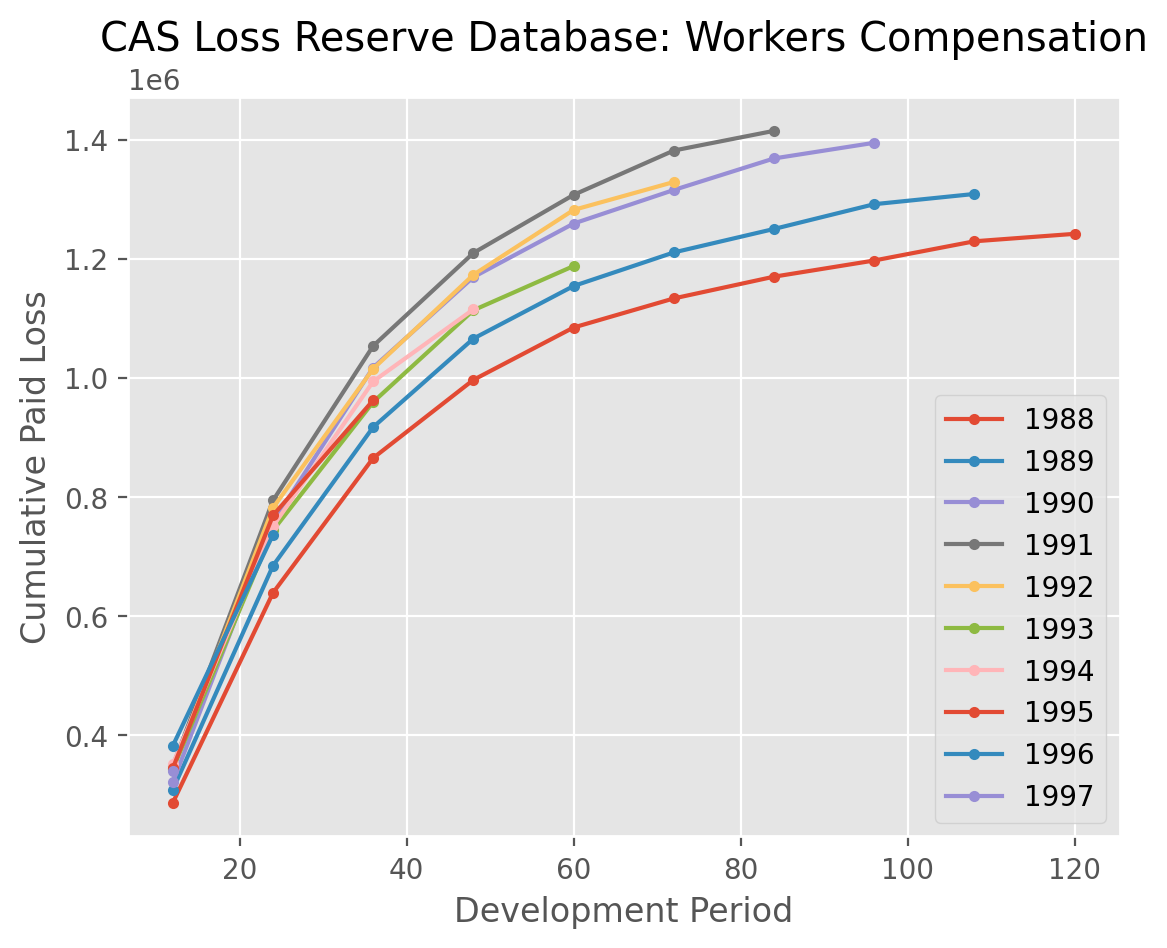
Exposing Pandas functionality#
The ability to move from a triangle to a pandas DataFrame opens up the full
suite of pandas functionality to you. For the more commonly used
functionality, we handle the to_frame() for you. For example,
triangle.to_frame().plot() is equivalent to triangle.plot().
cl.load_sample('clrd').groupby('LOB').sum().loc['wkcomp', 'CumPaidLoss'].T.plot(
    marker='.',
    title='CAS Loss Reserve Database: Workers Compensation').set(
    xlabel='Development Period', ylabel='Cumulative Paid Loss');
Many of the more commonly used pandas methods are passed through in this way allowing for working with triangles as DataFrames.
Aggregations |
IO |
Shaping |
Other |
|---|---|---|---|
|
|
|
|
|
|
|
|
|
|
|
|
|
|
|
|
|
|
|
|
|
|
|
|
|
|
||
|
|||
|
|||
|
Note
While some of these methods have been rewritten to return a Triangle, Many are pandas methods and will have return values consistent with pandas.
Accessors#
Like pandas .str and .dt accessor functions, you can also perform operations
on the origin, development or valuation of a triangle. For example, all
of these operations are legal.
raa = cl.load_sample('raa')
x = raa[raa.origin=='1986']
x = raa[(raa.development>=24)&(raa.development<=48)]
x = raa[raa.origin<='1985-JUN']
x = raa[raa.origin>'1987-01-01'][raa.development<=36]
x = raa[raa.valuation<raa.valuation_date]
These accessors apply boolean filtering along the origin or development of the
triangle. Because boolean filtering can only work on one axis at a time, you may
need to split up your indexing to achieve a desired result.
# Illegal use of boolean filtering of two different axes
x = raa[(raa.origin>'1987-01-01')&(raa.development<=36)]
# Instead, chain the boolean filters together.
x = raa[raa.origin>'1987-01-01'][raa.development<=36]
When using the accessors to filter a triangle, you may be left with empty portions
of the triangle that need to be trimmed up. The dropna method will look for
any origin periods or development periods that are fully empty at the edges
of the triangle and eliminate them for you.
raa = cl.load_sample('raa')
raa[raa.origin>'1987-01-01']
| 12 | 24 | 36 | 48 | 60 | 72 | 84 | 96 | 108 | 120 | |
|---|---|---|---|---|---|---|---|---|---|---|
| 1988 | 1,351 | 6,947 | 13,112 | |||||||
| 1989 | 3,133 | 5,395 | ||||||||
| 1990 | 2,063 |
There are many more methods available to manipulate triangles. The complete
list of methods is available under the Triangle docstrings.