Development#
Basics and Commonalities#
Before stepping into fitting development patterns, its worth reviewing the basics of Estimators. The main modeling API implemented by chainladder follows that of the scikit-learn estimator. An estimator is any object that learns from data.
Scikit-Learn API#
The scikit-learn API is a common modeling interface that is used to construct and
fit a countless variety of machine learning algorithms. The common interface
allows for very quick swapping between models with minimal code changes. The
chainladder package has adopted the interface to promote a standardized approach
to fitting reserving models.
All estimator objects can optionally be configured with parameters to uniquely specify the model being built. This is done ahead of pushing any data through the model.
estimator = Estimator(param1=1, param2=2)
All estimator objects expose a fit method that takes a Triangle as input, X:
estimator.fit(X=data)
All estimators include a sample_weight option to the fit method to specify
an exposure basis. If an exposure base is not applicable, then this argument is
ignored.
estimator.fit(X=data, sample_weight=weight)
All estimators either transform the input Triangle or predict an outcome.
Transformers#
All transformers include a transform method. The method is used to transform a
Triangle and it will always return a Triangle with added features based on the
specifics of the transformer.
transformed_data = estimator.transform(data)
Other than final IBNR models, chainladder estimators are transformers.
That is, they return your Triangle back to you with additional properties.
Transforming can be done at the time of fit.
# Fitting and Transforming
estimator.fit(data)
transformed_data = estimator.transform(data)
# One line equivalent
transformed_data = estimator.fit_transform(data)
assert isinstance(transformed_data, cl.Triangle)
Predictors#
All predictors include a predict method.
prediction = estimator.predict(new_data)
Predictors are intended to create new predictions. It is not uncommon to fit a model on a more aggregate view, say national level, of data and predict on a more granular triangle, state or provincial.
Parameter Types#
Estimator parameters: All the parameters of an estimator can be set when it is
instantiated or by modifying the corresponding attribute. These parameters
define how you’d like to fit an estimator and are chosen before the fitting
process. These are often referred to as hyperparameters in the context of
Machine Learning, and throughout these documents. Most of the hyperparameters
of the chainladder package take on sensible defaults.
estimator = Estimator(param1=1, param2=2)
assert estimator.param1 == 1
Estimated parameters: When data is fitted with an estimator, parameters are estimated from the data at hand. All the estimated parameters are attributes of the estimator object ending by an underscore. The use of the underscore is a key API design style of scikit-learn that allows for the quicker recognition of fitted parameters vs hyperparameters:
estimator.estimated_param_
In many cases the estimated parameters are themselves Triangles and can be
manipulated using the same methods we learned about in the Triangle class.
import chainladder as cl
import pandas as pd
import matplotlib.pyplot as plt
plt.style.use('ggplot')
%config InlineBackend.figure_format = 'retina'
dev = cl.Development().fit(cl.load_sample('ukmotor'))
type(dev.cdf_)
chainladder.core.triangle.Triangle
Commonalities#
All “Development Estimators” are transformers and reveal common a set of properties when they are fit.
ldf_represents the fitted age-to-age factors of the model.cdf_represents the fitted age-to-ultimate factors of the model.All “Development estimators” implement the
transformmethod.
cdf_ is nothing more than the cumulative representation of the ldf_ vectors.
dev = cl.Development().fit(cl.load_sample('raa'))
dev.ldf_.incr_to_cum() == dev.cdf_
True
Development#
Development allows for the selection of loss development patterns. Many
of the typical averaging techniques are available in this class: simple,
volume and regression through the origin. Additionally, Development
includes patterns to allow for fine-tuned exclusion of link-ratios from the LDF
calculation.
raa = cl.load_sample('raa')
cl.Development(average='simple')
Development(average='simple')In a Jupyter environment, please rerun this cell to show the HTML representation or trust the notebook.
On GitHub, the HTML representation is unable to render, please try loading this page with nbviewer.org.
Development(average='simple')
Alternatively, you can provide a list to parameterize each development period
separately. When adjusting individual development periods the list must be
the same length as your triangles link_ratio development axis.
len(raa.link_ratio.development)
9
cl.Development(average=['volume']+['simple']*8)
Development(average=['volume', 'simple', 'simple', 'simple', 'simple', 'simple',
                     'simple', 'simple', 'simple'])
In a Jupyter environment, please rerun this cell to show the HTML representation or trust the notebook. On GitHub, the HTML representation is unable to render, please try loading this page with nbviewer.org.
Development(average=['volume', 'simple', 'simple', 'simple', 'simple', 'simple',
                     'simple', 'simple', 'simple'])
This approach works for average, n_periods, drop_high and drop_low.
Notice where you have not specified a parameter, a sensible default is chosen for you.
Omitting link ratios#
There are several arguments for dropping individual cells from the triangle as well as excluding whole valuation periods or highs and lows. Any combination of the ‘drop’ arguments is permissible.
cl.Development(
    drop_high=[True]*5+[False]*4,
    drop_low=[True]*5+[False]*4).fit(raa)
Development(drop_high=[True, True, True, True, True, False, False, False,
                       False],
            drop_low=[True, True, True, True, True, False, False, False, False])
In a Jupyter environment, please rerun this cell to show the HTML representation or trust the notebook. On GitHub, the HTML representation is unable to render, please try loading this page with nbviewer.org.
Development(drop_high=[True, True, True, True, True, False, False, False,
                       False],
drop_low=[True, True, True, True, True, False, False, False, False])cl.Development(drop_valuation='1985').fit(raa)
Development(drop_valuation='1985')In a Jupyter environment, please rerun this cell to show the HTML representation or trust the notebook.
On GitHub, the HTML representation is unable to render, please try loading this page with nbviewer.org.
Development(drop_valuation='1985')
cl.Development(drop=[('1985', 12), ('1987', 24)]).fit(raa)
Development(drop=[('1985', 12), ('1987', 24)])In a Jupyter environment, please rerun this cell to show the HTML representation or trust the notebook. On GitHub, the HTML representation is unable to render, please try loading this page with nbviewer.org.
Development(drop=[('1985', 12), ('1987', 24)])cl.Development(drop=('1985', 12), drop_valuation='1988').fit(raa)
Development(drop=('1985', 12), drop_valuation='1988')In a Jupyter environment, please rerun this cell to show the HTML representation or trust the notebook. On GitHub, the HTML representation is unable to render, please try loading this page with nbviewer.org.
Development(drop=('1985', 12), drop_valuation='1988')When using drop, the earliest age of the link_ratio should be referenced.
For example, use 12 to drop the 12-24 ratio.
Note
drop_high and drop_low are ignored in cases where the number of link ratios available for a given development period is less than 1.
Extended Link Ratio Family#
The Development estimator is based on the regression framework known as the
Extended Link Ratio Family (ELRF). A nice property of this family is that we
not only get estimates for our patterns (cdf_, and ldf_), but also
measures of variability of our estimates (sigma_, std_err_ and std_residuals_
). These variability properties are used to develop the stochastic features in the
MackChainladder method, but even for deterministic methods these variability
estimates can be used as a diagnostic tool to validate the appropriateness of using
multiplicative link ratios.
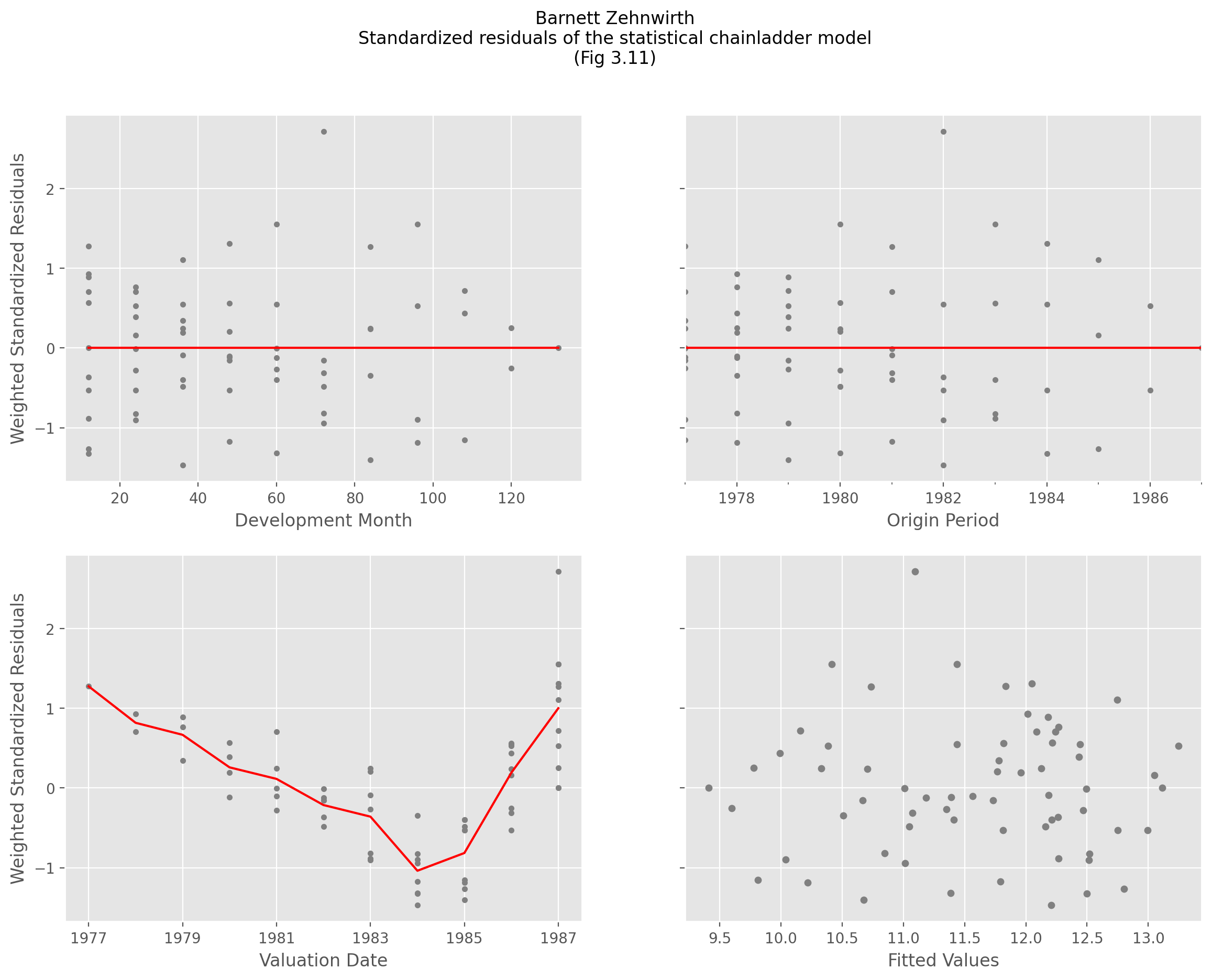
The std_residuals_ in particular is described by Barnett and Zehnwirth as a diagnostic
that points to the inferiority of the chainladder method relative to the probablistic
trend family.
raa = cl.load_sample('raa')
model = cl.Development().fit(raa)
model.std_residuals_
| 12 | 24 | 36 | 48 | 60 | 72 | 84 | 96 | 108 | |
|---|---|---|---|---|---|---|---|---|---|
| 1981 | -0.5722 | -0.8317 | -0.7489 | -0.3442 | 0.8704 | 1.4143 | -0.0003 | -0.6819 | |
| 1982 | 2.3075 | -0.7161 | 1.9716 | 1.5900 | 0.1982 | -0.9488 | 1.0919 | 0.7315 | |
| 1983 | -0.1267 | -0.2299 | -0.4811 | -0.1780 | 0.9056 | -0.2967 | -0.8987 | ||
| 1984 | -0.4305 | -0.8365 | 0.3723 | -1.3074 | 0.0012 | -0.1064 | |||
| 1985 | 1.1398 | 0.0943 | 0.6175 | -0.0170 | -1.5437 | ||||
| 1986 | 0.2936 | 0.4633 | -0.6809 | 0.7825 | |||||
| 1987 | 0.5961 | 2.0935 | -0.5805 | ||||||
| 1988 | 0.4717 | 0.6607 | |||||||
| 1989 | -0.4282 |
Replicating Fig 2.6 from their paper can be accomplished with a bit of manipulation of the residual triangles.
Show code cell source
fig, ((ax00, ax01), (ax10, ax11)) = plt.subplots(ncols=2, nrows=2, figsize=(10,8))
model.std_residuals_.T.plot(
    style='.', color='gray', legend=False, grid=True, ax=ax00,
    xlabel='Development Month', ylabel='Weighted Standardized Residuals')
model.std_residuals_.iloc[..., :-1].mean('origin').T.plot(
    color='red', legend=False, grid=True, ax=ax00)
model.std_residuals_.plot(
    style='.', color='gray', legend=False, grid=True, ax=ax01, xlabel='Origin Period')
model.std_residuals_.mean('development').plot(
    color='red', legend=False, grid=True, ax=ax01)
model.std_residuals_.dev_to_val().T.plot(
    style='.', color='gray', legend=False, grid=True, ax=ax10,
    xlabel='Valuation Date', ylabel='Weighted Standardized Residuals')

model.std_residuals_.dev_to_val().mean('origin').T.plot(color='red', legend=False, grid=True, ax=ax10)
pd.concat((
    (raa[raa.valuation<raa.valuation_date]*model.ldf_.values).unstack().rename('Fitted Values'),
    model.std_residuals_.unstack().rename('Residual')), axis=1).dropna().plot(
    kind='scatter', marker='o', color='gray', x='Fitted Values', y='Residual', ax=ax11, grid=True, sharey=True)
fig.suptitle("Barnett Zehnwirth\nStandardized residuals of the Extended Link Ratio Family (ELRF)\n(Fig 2.6)");
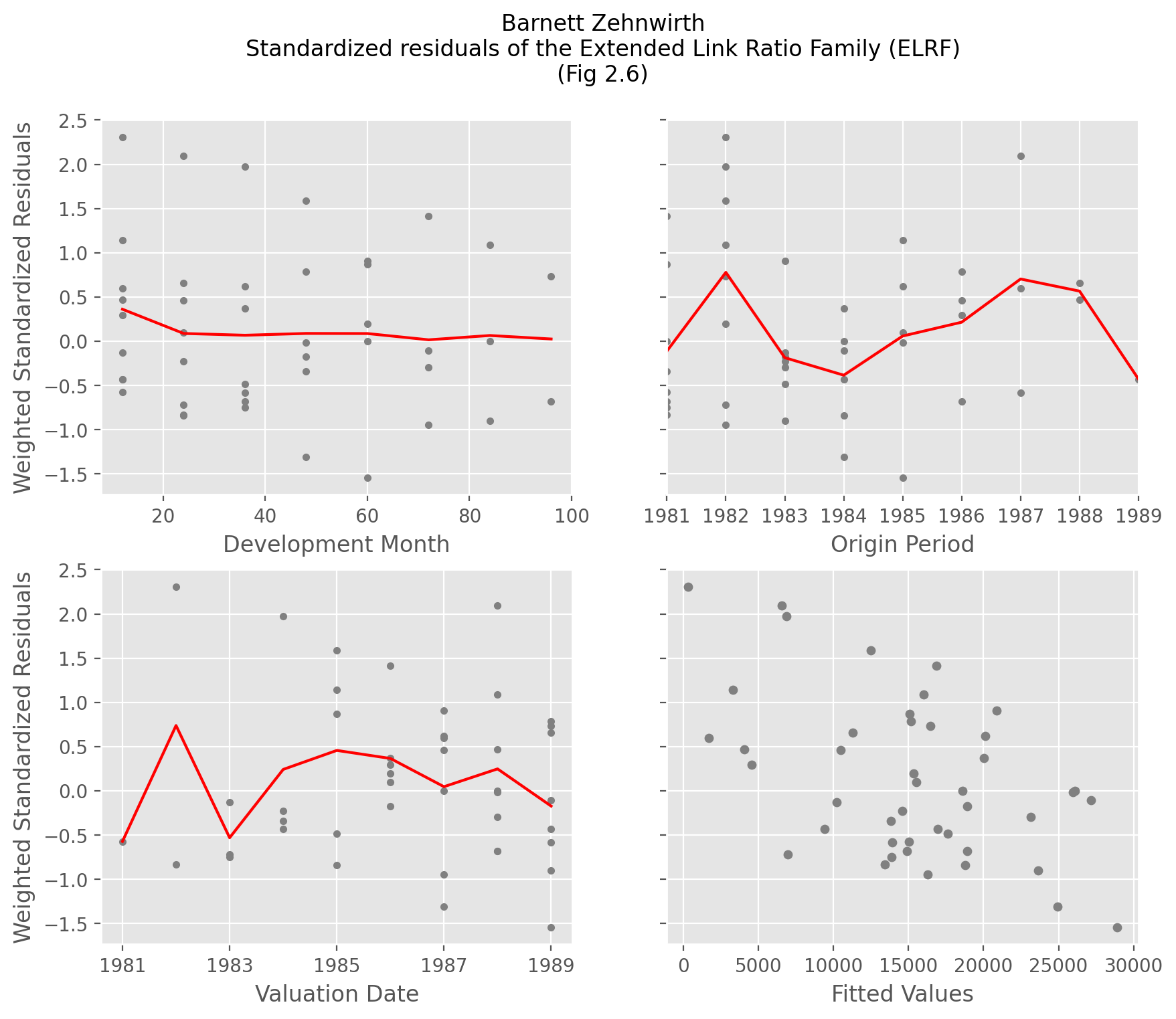
These residual plots which should should look random are used to highlight whether the chainladder model is violated. Violations generally occur due to trends in the valuation axis which are not accounted for in the basic chainladder method.
Transforming#
When transforming a Triangle, you will receive a copy of the original
triangle back along with the fitted properties of the Development
estimator. Where the original Triangle contains all link ratios, the transformed
version recognizes any ommissions you specify.
triangle = cl.load_sample('raa')
dev = cl.Development(drop=('1982', 12), drop_valuation='1988')
transformed_triangle = dev.fit_transform(triangle)
transformed_triangle.ldf_
| 12-24 | 24-36 | 36-48 | 48-60 | 60-72 | 72-84 | 84-96 | 96-108 | 108-120 | |
|---|---|---|---|---|---|---|---|---|---|
| (All) | 2.6625 | 1.5447 | 1.2975 | 1.1719 | 1.1134 | 1.0468 | 1.0294 | 1.0331 | 1.0092 |
transformed_triangle.link_ratio.heatmap()
| 12-24 | 24-36 | 36-48 | 48-60 | 60-72 | 72-84 | 84-96 | 96-108 | 108-120 | |
|---|---|---|---|---|---|---|---|---|---|
| 1981 | 1.6498 | 1.3190 | 1.0823 | 1.1469 | 1.1951 | 1.1130 | 1.0333 | 1.0092 | |
| 1982 | 1.2593 | 1.9766 | 1.2921 | 1.1318 | 0.9934 | 1.0331 | |||
| 1983 | 2.6370 | 1.5428 | 1.1635 | 1.1607 | 1.1857 | 1.0264 | |||
| 1984 | 2.0433 | 1.3644 | 1.3489 | 1.1015 | 1.0377 | ||||
| 1985 | 8.7592 | 1.6556 | 1.3999 | 1.0087 | |||||
| 1986 | 4.2597 | 1.8157 | 1.2255 | ||||||
| 1987 | 7.2172 | 1.1250 | |||||||
| 1988 | 1.8874 | ||||||||
| 1989 | 1.7220 |
By decoupling the fit and transform methods, we can apply our Development
estimator to new data. This is a common pattern of the scikit-learn API. In this
example we generate development patterns at an industry level and apply those
patterns to individual companies.
clrd = cl.load_sample('clrd')
clrd = clrd[clrd['LOB']=='wkcomp']['CumPaidLoss']
# Summarize Triangle to industry level to estimate patterns
dev = cl.Development().fit(clrd.sum())
# Apply Industry patterns to individual companies
dev.transform(clrd)
| Triangle Summary | |
|---|---|
| Valuation: | 1997-12 |
| Grain: | OYDY |
| Shape: | (132, 1, 10, 10) |
| Index: | [GRNAME, LOB] |
| Columns: | [CumPaidLoss] |
Groupby#
Triangles have a groupby method that follows pandas syntax and this allows for aggregating
triangle data to a more reasonable level for any particular analysis. However, it is often
the desire of an actuary to estimate development factors at a more aggregate grain generally
and then apply it to a more detailed triangle.
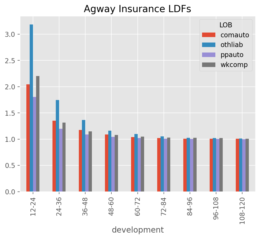
We can, for example, pick volume-weighted development patterns at a Line of Business level and subsequently apply them to each company within the line of business as follows:
clrd = cl.load_sample('clrd')['CumPaidLoss']
clrd = cl.Development(groupby='LOB').fit_transform(clrd)

clrd.shape, clrd.ldf_.shape
((775, 1, 10, 10), (6, 1, 1, 9))
Notice we’ve retained the grain of the original triangle, but there are six sets of development patterns, one for each line of business. Using this transformed triangle in an IBNR esimtator will result in IBNR at the original grain but using patterns at the Line of Business grain.
It is worth noting that fitting and transforming are entirely decoupled from one another, and we could achieve the same outcome by directly aggregating the Triangle before passing to the fit method.
clrd = cl.load_sample('clrd')['CumPaidLoss']
model = cl.Development().fit(clrd.groupby('LOB').sum())
clrd = model.transform(clrd)

clrd.shape, clrd.ldf_.shape
((775, 1, 10, 10), (6, 1, 1, 9))
This begs the question, why do we need a groupby hyperparameter as part of the Development estimator when we can aggregate the Triangle before fitting? In more advanced situations, we will be creating compound estimators called Pipelines which are very powerful for building custom workflows, but with the limitation that
fitting and transforming have to be coupled together. You can explore this in more detail in the
Pipeline section.
DevelopmentConstant#
The DevelopmentConstant estimator simply allows you to hard code development
patterns into a Development Estimator. A common example would be to include a
set of industry development patterns in your workflow that are not directly
estimated from any of your own data.
triangle = cl.load_sample('ukmotor')
patterns={12: 2, 24: 1.25, 36: 1.1, 48: 1.08, 60: 1.05, 72: 1.02}
cl.DevelopmentConstant(patterns=patterns, style='ldf').fit(triangle).ldf_
| 12-24 | 24-36 | 36-48 | 48-60 | 60-72 | 72-84 | |
|---|---|---|---|---|---|---|
| (All) | 2.0000 | 1.2500 | 1.1000 | 1.0800 | 1.0500 | 1.0200 |
By wrapping patterns in the DevelopmentConstant estimator, we can integrate
into a larger workflow with tail extrapolation and IBNR calculations.
Examples#
IncrementalAdditive#
The IncrementalAdditive method uses both the triangle of incremental
losses and the exposure vector for each accident year as a base. Incremental
additive ratios are computed by taking the ratio of incremental loss to the
exposure (which has been adjusted for the measurable effect of inflation), for
each accident year. This gives the amount of incremental loss in each year and
at each age expressed as a percentage of exposure, which we then use to square
the incremental triangle.
tri = cl.load_sample("ia_sample")
ia = cl.IncrementalAdditive().fit(
    X=tri['loss'],
    sample_weight=tri['exposure'].latest_diagonal)
ia.incremental_.round(0)
| 12 | 24 | 36 | 48 | 60 | 72 | |
|---|---|---|---|---|---|---|
| 2000 | 1,001.00 | 854.00 | 568.00 | 565.00 | 347.00 | 148.00 |
| 2001 | 1,113.00 | 990.00 | 671.00 | 648.00 | 422.00 | 164.00 |
| 2002 | 1,265.00 | 1,168.00 | 800.00 | 744.00 | 482.00 | 195.00 |
| 2003 | 1,490.00 | 1,383.00 | 1,007.00 | 849.00 | 543.00 | 220.00 |
| 2004 | 1,725.00 | 1,536.00 | 1,068.00 | 984.00 | 629.00 | 255.00 |
| 2005 | 1,889.00 | 1,811.00 | 1,256.00 | 1,157.00 | 740.00 | 300.00 |
These incremental_ values are then used to determine an implied set of
mutiplicative development patterns. Because incremental additive values are
unique for each origin, so too will be the ldf_.
ia.ldf_
| 12-24 | 24-36 | 36-48 | 48-60 | 60-72 | |
|---|---|---|---|---|---|
| 2000 | 1.8531 | 1.3062 | 1.2332 | 1.1161 | 1.0444 |
| 2001 | 1.8895 | 1.3191 | 1.2336 | 1.1233 | 1.0426 |
| 2002 | 1.9233 | 1.3288 | 1.2301 | 1.1212 | 1.0438 |
| 2003 | 1.9282 | 1.3505 | 1.2188 | 1.1148 | 1.0418 |
| 2004 | 1.8904 | 1.3276 | 1.2274 | 1.1184 | 1.0429 |
| 2005 | 1.9586 | 1.3395 | 1.2335 | 1.1210 | 1.0438 |
Incremental calculation#
The estimation of the incremental triangle can be done with varying hyperparameters
of n_period and average similar to the Development estimator. Additionally,
a trend in the origin period can also be selected.
Suppose there is a vector zeta_ that represents an estimate of the incremental
losses, X for a development period as a percentage of some exposure or sample_weight.
Using a ‘volume’ weighted estimate for all origin periods, we can manually estimate zeta_.
zeta_ = tri['loss'].cum_to_incr().sum('origin') / tri['exposure'].sum('origin')
zeta_
| 12 | 24 | 36 | 48 | 60 | 72 | |
|---|---|---|---|---|---|---|
| 2000 | 0.2432 | 0.2220 | 0.1540 | 0.1419 | 0.0907 | 0.0368 |
The zeta_ vector along with the sample_weight and optionally a trend
are used to propagate incremental losses to the lower half of the Triangle.
In the trivial case of no trend, we can estimate the incrementals for age 72.
zeta_.loc[..., 72] * tri['exposure'].latest_diagonal
| 72 | |
|---|---|
| 2000 | 148.00 |
| 2001 | 163.85 |
| 2002 | 195.43 |
| 2003 | 220.11 |
| 2004 | 255.15 |
| 2005 | 299.97 |
These are the same incrementals that the IncrementalAdditive method produces.
zeta_.loc[..., 72]*tri['exposure'].latest_diagonal == ia.incremental_.loc[..., 72]
True
Trending#
The IncrementalAdditive method supports trending through the trend
and the future_trend hyperparameters. The trend parameter is used in the
fitting of zeta_ and it trends all inner diagonals of the Triangle to its
latest_diagonal before estimating zeta_.
The future_trend hyperparameter is used to trend beyond the latest_diagonal
into the lower half of the Triangle. If no future trend is supplied, then
the future_trend is assumed to be that of the trend parameter.
cl.IncrementalAdditive(trend=0.02, future_trend=0.05).fit(
    X=tri['loss'],
    sample_weight=tri['exposure'].latest_diagonal
).incremental_.round(0)
| 12 | 24 | 36 | 48 | 60 | 72 | |
|---|---|---|---|---|---|---|
| 2000 | 1,001.00 | 854.00 | 568.00 | 565.00 | 347.00 | 148.00 |
| 2001 | 1,113.00 | 990.00 | 671.00 | 648.00 | 422.00 | 172.00 |
| 2002 | 1,265.00 | 1,168.00 | 800.00 | 744.00 | 511.00 | 215.00 |
| 2003 | 1,490.00 | 1,383.00 | 1,007.00 | 908.00 | 604.00 | 255.00 |
| 2004 | 1,725.00 | 1,536.00 | 1,151.00 | 1,105.00 | 735.00 | 310.00 |
| 2005 | 1,889.00 | 1,967.00 | 1,420.00 | 1,364.00 | 907.00 | 383.00 |
Note
These trend assumptions are applied to the incremental Triangle which produces drastically different answers from the same trends applied to a cumulative Triangle.
A nice property of this estimator is that it really only requires incremental amounts
so a Triangle that has cumulative data censored data in earlier diagonals can
leverage this method. Another nice property is that it allows for more explicit recognition
of future inflation in your estimate via the trend factor.
MunichAdjustment#
The MunichAdjustment is a bivariate adjustment to loss development factors.
There is a fundamental correlation between the paid and the case incurred data
of a triangle. The ratio of paid to incurred (P/I) has information that can
be used to simultaneously adjust the basic development factor selections for the
two separate triangles.
Depending on whether the momentary (P/I) ratio is below or above average,
one should use an above-average or below-average paid development factor and/or
a below-average or above-average incurred development factor. In doing so, the
model replaces a set of development patterns that would be used for all
origins with individualized development curves that reflect the unique levels
of (P/I) per origin period.
BerquistSherman Comparison#
This method is similar to the BerquistSherman approach in that it tries to
adjust for case reserve adequacy. However it is different in two distinct ways.
The
BerquistShermanmethod is a direct adjustment to the data whereas the MunichAdjustment keeps theTriangleintact and adjusts the development patterns.The MunichAdjustment is built in the context of a stochastic framework.
Residuals#
The MunichAdjustment uses the correlation between the residuals of the
univariate (basic) model and the (P/I) model. These correlations spin off a
property lambda_ which is represented by the line through the origin of
the correlation plots.
With the correlations, lambda_ known, the basic development patterns can
be adjusted based on the (P/I) ratio at any given cell of the Triangle.
Examples#
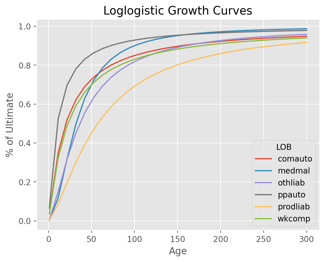
ClarkLDF#
ClarkLDF estimates growth curves of the form ‘loglogistic’ or ‘weibull’
for the incremental loss development of a Triangle. These growth curves are
monotonic increasing and are more relevant for paid data. While the model can
be used for case incurred data, if there is too much “negative” development,
other Estimators should be used.
The Loglogistic Growth Function:
$G(x|\omega, \theta) =\frac{x^{\omega }}{x^{\omega } + \theta^{\omega }}$
The Weibull Growth Function:
$G(x|\omega, \theta) =1-exp(-\left (\frac{x}{\theta} \right )^\omega)$
Parameterized growth curves can produce patterns for any age and can even be used to estimate a tail beyond the latest age in a Triangle. In general, the loglogistic growth curve produces a larger tail than the weibull growth curve.
LDF and Cape Cod methods#
Clark approaches curve fitting with two different methods, an LDF approach and a Cape Cod approach. The LDF approach only requires a loss triangle whereas the Cape Cod approach would also need a premium vector. Choosing between the two methods occurs at the time you fit the estimator. When a premium vector is included, the Cape Cod method is invoked.
A simple example of using ClarkLDF LDF Method. Upon fitting the Estimator,
we obtain both omega_ and theta_.
clrd = cl.load_sample('clrd').groupby('LOB').sum()
dev = cl.ClarkLDF(growth='weibull').fit(clrd['CumPaidLoss'])
dev.omega_
| CumPaidLoss | |
|---|---|
| LOB | |
| comauto | 0.928929 |
| medmal | 1.569649 |
| othliab | 1.330082 |
| ppauto | 0.831529 |
| prodliab | 1.456171 |
| wkcomp | 0.898279 |
Perhaps more useful than the parameters is the growth curve G_ function they
represent which can be used to deetermine the development factor at any age.
1/dev.G_(37.5).to_frame()
LOB
comauto     1.270899
medmal      1.707238
othliab     1.619168
ppauto      1.118801
prodliab    2.126153
wkcomp      1.311587
dtype: float64
Another example showing the usage of the ClarkLDF Cape Cod approach. With
the Cape Cod, an Expected Loss Ratio is included as an extra feature in the elr_ property.
cl.ClarkLDF().fit(
    X=clrd['CumPaidLoss'],
    sample_weight=clrd['EarnedPremDIR'].latest_diagonal
).elr_
| CumPaidLoss | |
|---|---|
| LOB | |
| comauto | 0.680325 |
| medmal | 0.701443 |
| othliab | 0.623806 |
| ppauto | 0.825932 |
| prodliab | 0.671024 |
| wkcomp | 0.697930 |
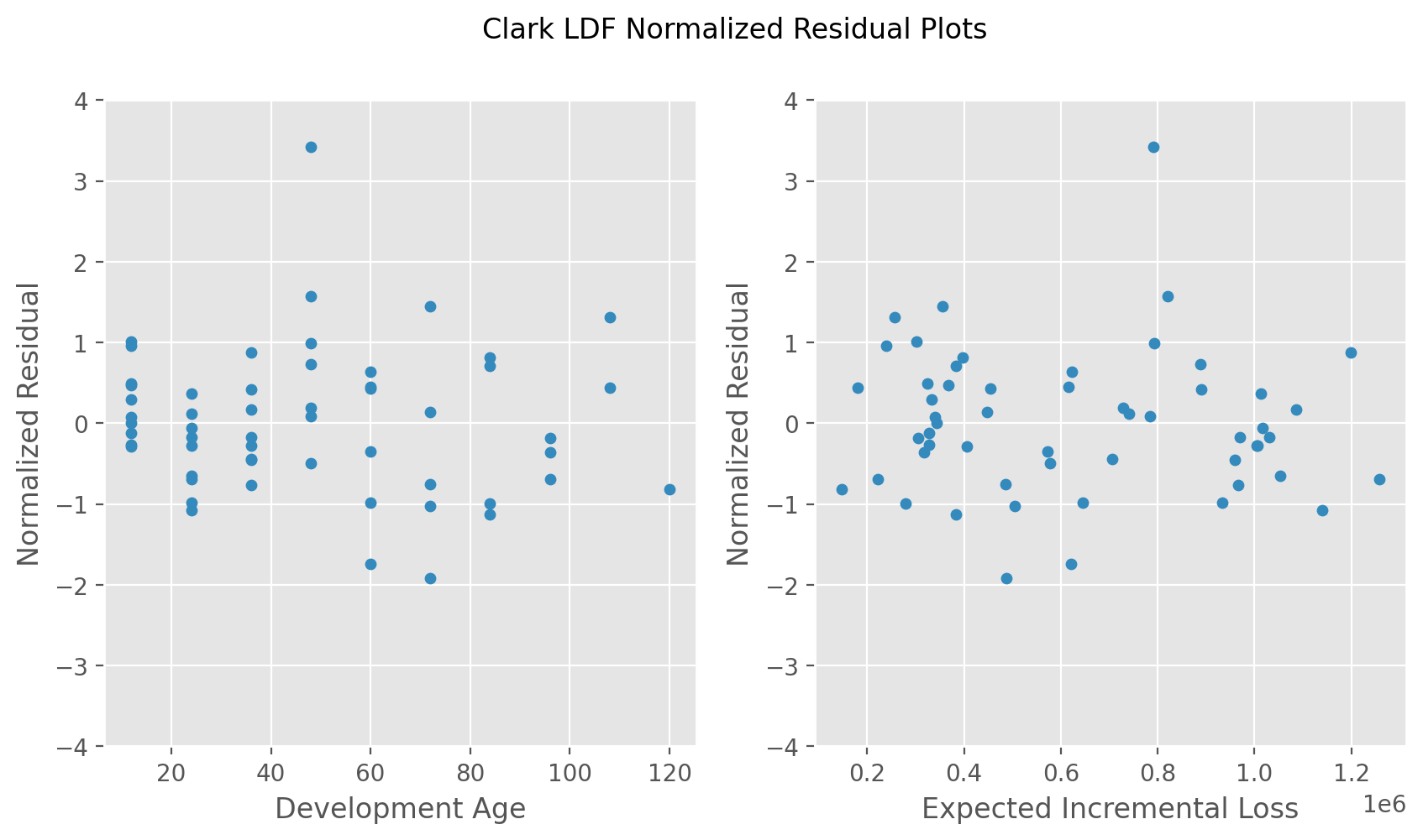
Residuals#
Clark’s model assumes Incremental losses are independent and identically distributed. To ensure compatibility with this assumption, he suggests reviewing the “Normalized Residuals” of the fitted incremental losses to ensure the assumption is not violated.
Stochastics#
Using MLE to solve for the growth curves, we can produce statistics about the parameter and process uncertainty of our model.
Examples#
CaseOutstanding#
The CaseOutstanding method is a deterministic method that estimates
incremental payment patterns from prior lag carried case reserves. Included
in this is also patterns for the carried case reserves based on the prior lag
carried case reserve.
Like the MunichAdjustment and BerquistSherman, this estimator
is useful when you want to incorporate information about case reserves into paid
ultimates.
To use it, a triangle with both paid and incurred amounts must be available.
tri = cl.load_sample('usauto')
model = cl.CaseOutstanding(paid_to_incurred=('paid', 'incurred')).fit(tri)
model.paid_ldf_
=== in _set_ldf ===
=== self.case ===
                12            24            36            48            60             72             84             96             108            120
1998  1.798098e+07  9.602188e+06  5.414189e+06  2.867316e+06  1.405073e+06  722000.560555  397562.100227  251150.266276  169222.000000   98117.000000
1999  1.968226e+07  1.051070e+07  5.926455e+06  3.138608e+06  1.538014e+06  790312.901593  435177.580406  274912.938466  185233.000000  107400.375016
2000  2.181513e+07  1.164970e+07  6.568678e+06  3.478725e+06  1.704682e+06  875955.506899  482335.790378  304704.000000  205305.855545  119038.863909
2001  1.904741e+07  1.017168e+07  5.735298e+06  3.037373e+06  1.488406e+06  764821.490526  421141.000000  266045.667404  179258.340423  103936.193801
2002  1.956232e+07  1.044665e+07  5.890341e+06  3.119483e+06  1.528642e+06  785497.000000  432525.754277  273237.711280  184104.252262  106745.913175
2003  2.091944e+07  1.117138e+07  6.298978e+06  3.335894e+06  1.634690e+06  839990.148108  462531.839581  292193.331822  196876.319229  114151.314922
2004  2.007969e+07  1.072294e+07  6.046125e+06  3.201985e+06  1.569070e+06  806271.365800  443964.942762  280464.142653  188973.333980  109569.066729
2005  2.039616e+07  1.089194e+07  6.141416e+06  3.252450e+06  1.593800e+06  818978.706486  450962.107761  284884.432846  191951.671841  111295.943707
2006  2.066376e+07  1.103484e+07  6.221991e+06  3.295122e+06  1.614710e+06  829723.593216  456878.667897  288622.076985  194470.051080  112756.131011
2007  2.162359e+07  1.154741e+07  6.511004e+06  3.448181e+06  1.689714e+06  868264.503103  478100.819120  302028.659070  203503.243309  117993.687132
=== self.paid ===
              12            24            36            48            60            72            84            96            108           120
1998  18539254.0  3.323104e+07  4.006201e+07  4.389204e+07  4.589654e+07  4.676542e+07  4.722132e+07  4.744688e+07  4.755546e+07  4.764419e+07
1999  20410193.0  3.609068e+07  4.325940e+07  4.715924e+07  4.920853e+07  5.016204e+07  5.062576e+07  5.087881e+07  5.100053e+07  5.109766e+07
2000  22120843.0  3.897601e+07  4.638928e+07  5.056238e+07  5.273528e+07  5.374010e+07  5.428433e+07  5.453322e+07  5.466649e+07  5.477415e+07
2001  22992259.0  4.009620e+07  4.776784e+07  5.209392e+07  5.436344e+07  5.537880e+07  5.587842e+07  5.611147e+07  5.622784e+07  5.632183e+07
2002  24092782.0  4.179531e+07  4.990380e+07  5.435288e+07  5.675438e+07  5.780722e+07  5.829581e+07  5.853516e+07  5.865467e+07  5.875120e+07
2003  24084451.0  4.139961e+07  4.907033e+07  5.358420e+07  5.593065e+07  5.697291e+07  5.749540e+07  5.775136e+07  5.787916e+07  5.798239e+07
2004  24369770.0  4.148986e+07  4.923668e+07  5.377467e+07  5.600590e+07  5.700632e+07  5.750783e+07  5.775352e+07  5.787618e+07  5.797527e+07
2005  25100697.0  4.270223e+07  5.064499e+07  5.499527e+07  5.726166e+07  5.827785e+07  5.878727e+07  5.903682e+07  5.916142e+07  5.926207e+07
2006  25608776.0  4.360650e+07  5.144103e+07  5.584838e+07  5.814450e+07  5.917403e+07  5.969013e+07  5.994296e+07  6.006919e+07  6.017116e+07
2007  27229969.0  4.545463e+07  5.365308e+07  5.826515e+07  6.066793e+07  6.174527e+07  6.228535e+07  6.254992e+07  6.268202e+07  6.278873e+07
=== set LDF return ===
             Triangle Summary
Valuation:           2261-12
Grain:                  OYDY
Shape:         (1, 2, 10, 9)
Index:               [Total]
Columns:    [incurred, paid]
| 24-36 | 36-48 | 48-60 | 60-72 | 72-84 | 84-96 | 96-108 | 108-120 | 120-132 | |
|---|---|---|---|---|---|---|---|---|---|
| (All) | 0.8428 | 0.7100 | 0.7084 | 0.6968 | 0.6376 | 0.6220 | 0.5534 | 0.4374 | 0.5243 |
In the example above, the incremental paid losses during the period 12-24 is expected to be
84.28% of the outstanding case reserve at lag 12. The set of patterns produced by
CaseOutstanding don’t follow the multiplicative approach commonly used in the
various IBNR methods making them not directly usable. Because of this, the estimator
determines the ‘implied’ multiplicative pattern so that a broader set of IBNR
methods can be used. Due to the origin period specifics on case reserves, each
origin gets its own set of multiplicative ldf_ patterns.
model.ldf_['paid']
| 12-24 | 24-36 | 36-48 | 48-60 | 60-72 | 72-84 | 84-96 | 96-108 | 108-120 | |
|---|---|---|---|---|---|---|---|---|---|
| 1998 | 1.7925 | 1.2056 | 1.0956 | 1.0457 | 1.0189 | 1.0097 | 1.0048 | 1.0023 | 1.0019 |
| 1999 | 1.7683 | 1.1986 | 1.0902 | 1.0435 | 1.0194 | 1.0092 | 1.0050 | 1.0024 | 1.0019 |
| 2000 | 1.7620 | 1.1902 | 1.0900 | 1.0430 | 1.0191 | 1.0101 | 1.0046 | 1.0024 | 1.0020 |
| 2001 | 1.7439 | 1.1913 | 1.0906 | 1.0436 | 1.0187 | 1.0090 | 1.0042 | 1.0021 | 1.0017 |
| 2002 | 1.7348 | 1.1940 | 1.0892 | 1.0442 | 1.0186 | 1.0085 | 1.0041 | 1.0020 | 1.0016 |
| 2003 | 1.7189 | 1.1853 | 1.0920 | 1.0438 | 1.0186 | 1.0092 | 1.0045 | 1.0022 | 1.0018 |
| 2004 | 1.7025 | 1.1867 | 1.0922 | 1.0415 | 1.0179 | 1.0088 | 1.0043 | 1.0021 | 1.0017 |
| 2005 | 1.7012 | 1.1860 | 1.0859 | 1.0412 | 1.0177 | 1.0087 | 1.0042 | 1.0021 | 1.0017 |
| 2006 | 1.7028 | 1.1797 | 1.0857 | 1.0411 | 1.0177 | 1.0087 | 1.0042 | 1.0021 | 1.0017 |
| 2007 | 1.6693 | 1.1804 | 1.0860 | 1.0412 | 1.0178 | 1.0087 | 1.0042 | 1.0021 | 1.0017 |
Incremental patterns#
The incremental patterns of the CaseOutstanding method are avilable as
additional properties for review. They are the paid_to_prior_case_ and the
case_to_prior_case_. These are useful to review when deciding on the appropriate
hyperparameters for paid_n_periods and case_n_periods. Once you are satisfied
with your hyperparameter tuning, you can see the fitted selections in the
paid_ldf_ and case_ldf_ incremental patterns.
model.case_to_prior_case_
| 24-36 | 36-48 | 48-60 | 60-72 | 72-84 | 84-96 | 96-108 | 108-120 | 120-132 | |
|---|---|---|---|---|---|---|---|---|---|
| 1998 | 0.5378 | 0.5541 | 0.5253 | 0.4981 | 0.5329 | 0.5380 | 0.5877 | 0.6970 | 0.5798 |
| 1999 | 0.5368 | 0.5649 | 0.5442 | 0.4969 | 0.5029 | 0.5800 | 0.6420 | 0.6506 | |
| 2000 | 0.5461 | 0.5742 | 0.5391 | 0.4872 | 0.5376 | 0.5432 | 0.6655 | ||
| 2001 | 0.5406 | 0.5660 | 0.5148 | 0.5013 | 0.5077 | 0.5414 | |||
| 2002 | 0.5409 | 0.5546 | 0.5406 | 0.4802 | 0.4881 | ||||
| 2003 | 0.5265 | 0.5765 | 0.5363 | 0.4764 | |||||
| 2004 | 0.5298 | 0.5665 | 0.5069 | ||||||
| 2005 | 0.5215 | 0.5539 | |||||||
| 2006 | 0.5261 | ||||||||
| 2007 |
model.case_ldf_
| 24-36 | 36-48 | 48-60 | 60-72 | 72-84 | 84-96 | 96-108 | 108-120 | 120-132 | |
|---|---|---|---|---|---|---|---|---|---|
| (All) | 0.5340 | 0.5638 | 0.5296 | 0.4900 | 0.5139 | 0.5506 | 0.6317 | 0.6738 | 0.5798 |
TweedieGLM#
The TweedieGLM implements the GLM reserving structure discussed by Taylor and McGuire.
A nice property of the GLM framework is that it is highly flexible in terms of including
covariates that may be predictive of loss reserves while maintaining a close relationship
to traditional methods. Additionally, the framework can be extended in a straightforward
way to incorporate various approaches to measuring prediction errors. Behind the
scenes, TweedieGLM is using scikit-learn’s TweedieRegressor estimator.
Long Format#
GLMs are fit to triangles in “Long Format”. That is, they are converted to pandas
DataFrames behind the scenes. Each axis of the Triangle is included in the
dataframe. The origin and development axes are in columns of the same name.
You can inspect what your Triangle looks like in long format by calling to_frame
with keepdims=True
cl.load_sample('clrd').to_frame(keepdims=True).reset_index().head()
| GRNAME | LOB | origin | development | IncurLoss | CumPaidLoss | BulkLoss | EarnedPremDIR | EarnedPremCeded | EarnedPremNet | |
|---|---|---|---|---|---|---|---|---|---|---|
| 0 | Adriatic Ins Co | othliab | 1995-01-01 | 12 | 8.0 | NaN | 8.0 | 139.0 | 131.0 | 8.0 |
| 1 | Adriatic Ins Co | othliab | 1995-01-01 | 24 | 11.0 | NaN | 4.0 | 139.0 | 131.0 | 8.0 |
| 2 | Adriatic Ins Co | othliab | 1995-01-01 | 36 | 7.0 | 3.0 | 4.0 | 139.0 | 131.0 | 8.0 |
| 3 | Adriatic Ins Co | othliab | 1996-01-01 | 12 | 40.0 | NaN | 40.0 | 410.0 | 359.0 | 51.0 |
| 4 | Adriatic Ins Co | othliab | 1996-01-01 | 24 | 40.0 | NaN | 40.0 | 410.0 | 359.0 | 51.0 |
Warning
‘origin’, ‘development’, and ‘valuation’ are reserved keywords for the dataframe. Declaring columns with these names separately will result in error.
While you can inspect the Triangle in long format, you will not directly convert
to long format yourself. The TweedieGLM does this for you. Additionally,
the origin of the design matrix is restated in years from the earliest origin
period. That is, is if the earliest origin is ‘1995-01-01’ then it gets replaced with
0. Consequently, ‘1996-04-01’ would be replaced with 1.25. This is done because
datetimes have limited support in scikit-learn. Finally, the TweedieGLM
will automatically convert the response to an incremental basis.
R-style formulas#
We use the patsy library to allow formulation of the the feature set X
of the GLM. Because X is a parameter that used extensively throughout
chainladder, the TweedieGLM refers to it as the design_matrix. Those
familiar with the R programming language will be familiar with the notation
used by patsy. For example, we can include both origin and development
as terms in a model.
genins = cl.load_sample('genins')
glm = cl.TweedieGLM(design_matrix='development + origin').fit(genins)
glm.coef_
| coef_ | |
|---|---|
| Intercept | 13.516322 |
| development | -0.006251 |
| origin | 0.033863 |
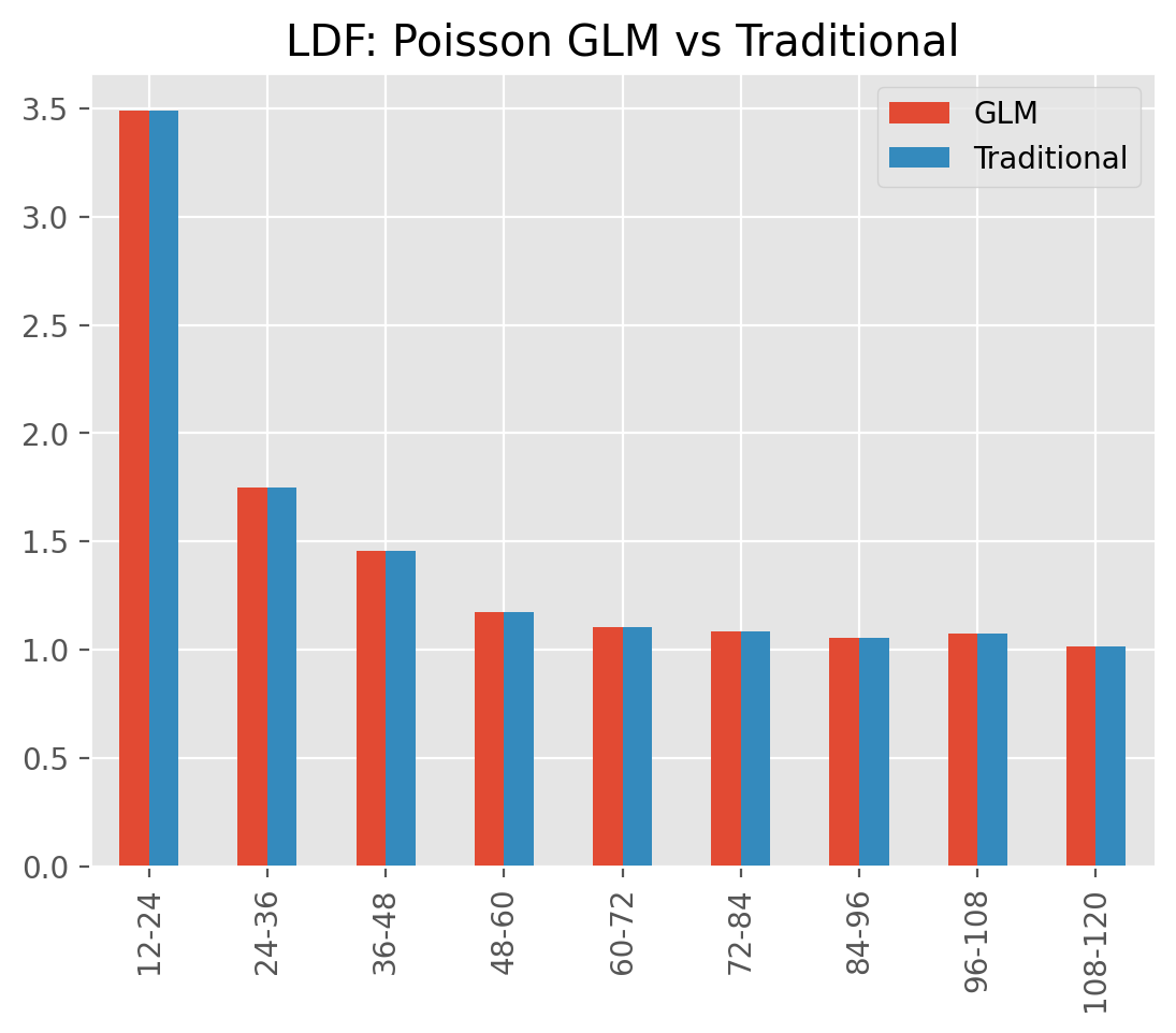
ODP Chainladder#
Replicating the results of the volume weighted chainladder development patterns
can be done by fitting a Poisson-log GLM to incremental paids. To do this, we
can specify the power and link of the estimator as well as the design_matrix.
The volume-weighted chainladder method can be replicated by including both
origin and development as categorical features.
dev = cl.TweedieGLM(
    design_matrix='C(development) + C(origin)',
    power=1, link='log').fit(genins)
A trivial comparison against the traditional Development estimator shows
a comparable set of ldf_ patterns.
Parsimonious modeling#
Having full access to all axes of the Triangle along with the powerful formulation
of patsy allows for substantial customization of the model fit. For example,
we can include ‘LOB’ interactions with piecewise linear coefficients to reduce
model complexity.
clrd = cl.load_sample('clrd')['CumPaidLoss'].groupby('LOB').sum()
clrd=clrd[clrd['LOB'].isin(['ppauto', 'comauto'])]
dev = cl.TweedieGLM(
    design_matrix='LOB+LOB:C(np.minimum(development, 36))+LOB:development+LOB:origin',
    max_iter=1000).fit(clrd)
dev.coef_
| coef_ | |
|---|---|
| Intercept | 12.550094 |
| LOB[T.ppauto] | 3.202525 |
| LOB[comauto]:C(np.minimum(development, 36))[T.24] | 0.578636 |
| LOB[ppauto]:C(np.minimum(development, 36))[T.24] | 0.449818 |
| LOB[comauto]:C(np.minimum(development, 36))[T.36] | 0.790583 |
| LOB[ppauto]:C(np.minimum(development, 36))[T.36] | 0.321155 |
| LOB[comauto]:development | -0.044631 |
| LOB[ppauto]:development | -0.054813 |
| LOB[comauto]:origin | 0.054570 |
| LOB[ppauto]:origin | 0.057791 |
This model is limited to 10 coefficients across two lines of business. The basic
chainladder model is known to be overparameterized with at least 18 parameters
requiring estimation. Despite drastically simplifying the model, the cdf_
patterns of the GLM are within 1% of the traditional chainladder for every lag
and for both lines of business:
((dev.cdf_.iloc[..., 0, :] /
  cl.Development().fit(clrd).cdf_) - 1
).to_frame().round(3)
| development | 12-Ult | 24-Ult | 36-Ult | 48-Ult | 60-Ult | 72-Ult | 84-Ult | 96-Ult | 108-Ult |
|---|---|---|---|---|---|---|---|---|---|
| LOB | |||||||||
| comauto | 0.002 | 0.003 | -0.01 | 0.003 | 0.011 | 0.008 | 0.005 | -0.000 | -0.002 |
| ppauto | 0.006 | 0.003 | -0.00 | 0.001 | 0.002 | 0.001 | 0.001 | 0.001 | 0.001 |
Like every other Development estimator, the TweedieGLM produces a set of ldf_
patterns and can be used in a larger workflow with tail extrapolation and reserve
estimation.
DevelopmentML#
DevelopmentML is a general development estimator that works as an interface to
scikit-learn compliant machine learning (ML) estimators. The TweedieGLM is
a special case of DevelopmentML with the ML algorithm limited to scikit-learn’s
TweedieRegressor estimator.
The Interface#
ML algorithms are designed to be fit against tabular data like a pandas DataFrame
or a 2D numpy array. A Triangle does not meet the definition and so DevelopmentML
is provided to incorporate ML into a broader reserving workflow. This includes:
Automatic conversion of Triangle to a dataframe for fitting
Flexibility in expressing any preprocessing as part of a scikit-learn
PipelinePredictions through the terminal development age of a
Triangleto fill in the lower halfPredictions converted to
ldf_patterns so that the results of the estimator are compliant with the rest ofchainladder, like tail selection and IBNR modeling.
Features#
Data from any axis of a Triangle is available to be used in the DevelopmentML
estimator. For example, we can use many of the scikit-learn components to
generate development patterns from both the time axes as well as the index of
the Triangle.
from sklearn.ensemble import RandomForestRegressor
from sklearn.pipeline import Pipeline
from sklearn.preprocessing import OneHotEncoder
from sklearn.compose import ColumnTransformer

clrd = cl.load_sample('clrd').groupby('LOB').sum()['CumPaidLoss']

# Decide how to preprocess the X (ML) dataset using sklearn
design_matrix = ColumnTransformer(transformers=[
    ('dummy', OneHotEncoder(drop='first'), ['LOB', 'development']),
    ('passthrough', 'passthrough', ['origin'])
])

# Wrap preprocessing and model in a larger sklearn Pipeline
estimator_ml = Pipeline(steps=[
    ('design_matrix', design_matrix),
    ('model', RandomForestRegressor())
])

# Fitting DevelopmentML fits the underlying ML model and gives access to ldf_
cl.DevelopmentML(estimator_ml=estimator_ml, y_ml='CumPaidLoss').fit(clrd).ldf_
| Triangle Summary | |
|---|---|
| Valuation: | 2261-12 |
| Grain: | OYDY |
| Shape: | (6, 1, 10, 9) |
| Index: | [LOB] |
| Columns: | [CumPaidLoss] |
Autoregressive#
The time-series nature of loss development naturally lends to an urge for autoregressive
features. That is, features that are based on predictions, albeit on a lagged basis.
DevelopmentML includes an autoregressive parameter that can be used to
express the response as a lagged feature as well.
Note
When using autoregressive features, you must also declare it as a column
in your estimator_ml Pipeline.
PatsyFormula#
While the sklearn preprocessing API is powerful, it can be tedious work with in
some instances. In particular, modeling complex interactions is much easier to do
with Patsy. The chainladder package includes a custom sklearn estimator
to gain access to the patsy API. This is done through the PatsyFormula estimator.
estimator_ml = Pipeline(steps=[
    ('design_matrix', cl.PatsyFormula('LOB:C(origin)+LOB:C(development)+development')),
    ('model', RandomForestRegressor())
])
cl.DevelopmentML(
    estimator_ml=estimator_ml,
    y_ml='CumPaidLoss').fit(clrd).ldf_.iloc[0, 0, 0].round(2)
| 12-24 | 24-36 | 36-48 | 48-60 | 60-72 | 72-84 | 84-96 | 96-108 | 108-120 | |
|---|---|---|---|---|---|---|---|---|---|
| (All) | 2.6100 | 1.4100 | 1.1900 | 1.1000 | 1.0400 | 1.0200 | 1.0100 | 1.0100 | 1.0100 |
Note
PatsyFormula is not an estimator designed to work with triangles. It is an sklearn transformer designed to work with pandas DataFrames allowing it to work directly in an sklearn Pipeline.
BarnettZehnwirth#
The BarnettZehnwirth estimator solves for development patterns using the
Probabilistic Trend Family (PTF) regression framework. Unlike the ELRF framework,
which assumes no valuation covariate, the PTF framework allows for this.
Structurally, the PTF regression is different from the ELRF (ELRF) regression framework in
two distinct ways:
Where the ELRF fits independent regressions to each adjacent development lag, the PTF regression is fit to the entire triangle
Where the ELRF is fit to cumulative amounts, the PTF is fit to the log of the incremental amounts of the
Triangle.
Formulation#
The PTF framework is an ordinary least squares (OLS) model with the response, y
being the log of the incremental amounts of a Triangle. These are assumed to be
normally distributed which implies the incrementals themselves are log-normal
distributed.
The framework includes coefficients for origin periods (alpha), development periods (gamma) and calendar period (iota).
$y(i, j) = \alpha {i} + \sum{k=1}^{j}\gamma {k}+ \sum{\iota =1}^{i+j}\gamma _{\iota}+ \varepsilon _{i,j}$
These coefficients can be categorical or continuous, and to support a wide range of model forms, patsy formulas are used.
abc = cl.load_sample('abc')

# Discrete origin, development, valuation
cl.BarnettZehnwirth(formula='C(origin)+C(development)').fit(abc).coef_.T
| Intercept | C(origin)[T.1.0] | C(origin)[T.2.0] | C(origin)[T.3.0] | C(origin)[T.4.0] | C(origin)[T.5.0] | C(origin)[T.6.0] | C(origin)[T.7.0] | C(origin)[T.8.0] | C(origin)[T.9.0] | ... | C(development)[T.24] | C(development)[T.36] | C(development)[T.48] | C(development)[T.60] | C(development)[T.72] | C(development)[T.84] | C(development)[T.96] | C(development)[T.108] | C(development)[T.120] | C(development)[T.132] | |
|---|---|---|---|---|---|---|---|---|---|---|---|---|---|---|---|---|---|---|---|---|---|
| coef_ | 11.836863 | 0.178824 | 0.345112 | 0.378133 | 0.405093 | 0.427041 | 0.431076 | 0.660383 | 0.963223 | 1.1568 | ... | 0.251091 | -0.055824 | -0.448589 | -0.828917 | -1.16913 | -1.507561 | -1.798345 | -2.0231 | -2.238333 | -2.427672 |
1 rows × 21 columns
# Linear coefficients for origin, development, and valuation
cl.BarnettZehnwirth(formula='origin+development+valuation').fit(abc).coef_.T
| Intercept | origin | development | valuation | |
|---|---|---|---|---|
| coef_ | 8.359157 | 4.215981 | 0.319288 | -4.116569 |
The PTF framework is particularly useful when there is calendar period inflation influences on loss development.