Applying Deterministic Methods

Getting Started

This tutorial focuses on using deterministic methods to square a triangle.

Be sure to make sure your packages are updated. For more info on how to update your pakages, visit Keeping Packages Updated.

# Black linter, optional
%load_ext lab_black

import pandas as pd
import numpy as np
import chainladder as cl
import matplotlib.pyplot as plt

print("pandas: " + pd.__version__)
print("numpy: " + np.__version__)
print("chainladder: " + cl.__version__)

pandas: 2.1.4
numpy: 1.24.3
chainladder: 0.8.18

Disclaimer

Note that a lot of the examples shown might not be applicable in a real world scenario, and is only meant to demonstrate some of the functionalities included in the package. The user should always follow all applicable laws, the Code of Professional Conduct, applicable Actuarial Standards of Practice, and exercise their best actuarial judgement.

Chainladder Method

The basic chainladder method is entirely specified by its development pattern selections. For this reason, the Chainladder estimator takes no additional assumptions, i.e. no additional arguments. Let’s start by loading an example dataset and creating an Triangle with Development patterns and a TailCurve. Recall, we can bundle these two estimators into a single Pipeline if we wish.

genins = cl.load_sample("genins")

genins_dev = cl.Pipeline(
    [("dev", cl.Development()), ("tail", cl.TailCurve())]
).fit_transform(genins)

We can now use the basic Chainladder estimator to estimate ultimate_ values of our Triangle.

genins_model = cl.Chainladder().fit(genins_dev)
genins_model.ultimate_

	2261
2001	4,016,553
2002	5,594,009
2003	5,537,497
2004	5,454,190
2005	5,001,513
2006	5,261,947
2007	5,827,759
2008	6,984,945
2009	5,808,708
2010	5,116,430

We can also view the ibnr_. Techincally the term IBNR is reserved for Incurred but not Reported, but the chainladder models use it to describe the difference between the ultimate and the latest evaluation period.

genins_model.ibnr_

	2261
2001	115,090
2002	254,924
2003	628,182
2004	865,922
2005	1,128,202
2006	1,570,235
2007	2,344,629
2008	4,120,447
2009	4,445,414
2010	4,772,416

It is often useful to see the completed Triangle and this can be accomplished by inspecting the full_triangle_. As with most other estimator properties, the full_triangle_ is itself a Triangle and can be manipulated as such.

genins

	12	24	36	48	60	72	84	96	108	120
2001	357,848	1,124,788	1,735,330	2,218,270	2,745,596	3,319,994	3,466,336	3,606,286	3,833,515	3,901,463
2002	352,118	1,236,139	2,170,033	3,353,322	3,799,067	4,120,063	4,647,867	4,914,039	5,339,085
2003	290,507	1,292,306	2,218,525	3,235,179	3,985,995	4,132,918	4,628,910	4,909,315
2004	310,608	1,418,858	2,195,047	3,757,447	4,029,929	4,381,982	4,588,268
2005	443,160	1,136,350	2,128,333	2,897,821	3,402,672	3,873,311
2006	396,132	1,333,217	2,180,715	2,985,752	3,691,712
2007	440,832	1,288,463	2,419,861	3,483,130
2008	359,480	1,421,128	2,864,498
2009	376,686	1,363,294
2010	344,014

genins_model.full_triangle_

	12	24	36	48	60	72	84	96	108	120	132	9999
2001	357,848	1,124,788	1,735,330	2,218,270	2,745,596	3,319,994	3,466,336	3,606,286	3,833,515	3,901,463	3,948,071	4,016,553
2002	352,118	1,236,139	2,170,033	3,353,322	3,799,067	4,120,063	4,647,867	4,914,039	5,339,085	5,433,719	5,498,632	5,594,009
2003	290,507	1,292,306	2,218,525	3,235,179	3,985,995	4,132,918	4,628,910	4,909,315	5,285,148	5,378,826	5,443,084	5,537,497
2004	310,608	1,418,858	2,195,047	3,757,447	4,029,929	4,381,982	4,588,268	4,835,458	5,205,637	5,297,906	5,361,197	5,454,190
2005	443,160	1,136,350	2,128,333	2,897,821	3,402,672	3,873,311	4,207,459	4,434,133	4,773,589	4,858,200	4,916,237	5,001,513
2006	396,132	1,333,217	2,180,715	2,985,752	3,691,712	4,074,999	4,426,546	4,665,023	5,022,155	5,111,171	5,172,231	5,261,947
2007	440,832	1,288,463	2,419,861	3,483,130	4,088,678	4,513,179	4,902,528	5,166,649	5,562,182	5,660,771	5,728,396	5,827,759
2008	359,480	1,421,128	2,864,498	4,174,756	4,900,545	5,409,337	5,875,997	6,192,562	6,666,635	6,784,799	6,865,853	6,984,945
2009	376,686	1,363,294	2,382,128	3,471,744	4,075,313	4,498,426	4,886,502	5,149,760	5,544,000	5,642,266	5,709,671	5,808,708
2010	344,014	1,200,818	2,098,228	3,057,984	3,589,620	3,962,307	4,304,132	4,536,015	4,883,270	4,969,825	5,029,196	5,116,430

genins_model.full_triangle_.dev_to_val()

	2001	2002	2003	2004	2005	2006	2007	2008	2009	2010	...	2012	2013	2014	2015	2016	2017	2018	2019	2020	2261
2001	357,848	1,124,788	1,735,330	2,218,270	2,745,596	3,319,994	3,466,336	3,606,286	3,833,515	3,901,463	...	3,948,071	3,948,071	3,948,071	3,948,071	3,948,071	3,948,071	3,948,071	3,948,071	3,948,071	4,016,553
2002		352,118	1,236,139	2,170,033	3,353,322	3,799,067	4,120,063	4,647,867	4,914,039	5,339,085	...	5,498,632	5,498,632	5,498,632	5,498,632	5,498,632	5,498,632	5,498,632	5,498,632	5,498,632	5,594,009
2003			290,507	1,292,306	2,218,525	3,235,179	3,985,995	4,132,918	4,628,910	4,909,315	...	5,378,826	5,443,084	5,443,084	5,443,084	5,443,084	5,443,084	5,443,084	5,443,084	5,443,084	5,537,497
2004				310,608	1,418,858	2,195,047	3,757,447	4,029,929	4,381,982	4,588,268	...	5,205,637	5,297,906	5,361,197	5,361,197	5,361,197	5,361,197	5,361,197	5,361,197	5,361,197	5,454,190
2005					443,160	1,136,350	2,128,333	2,897,821	3,402,672	3,873,311	...	4,434,133	4,773,589	4,858,200	4,916,237	4,916,237	4,916,237	4,916,237	4,916,237	4,916,237	5,001,513
2006						396,132	1,333,217	2,180,715	2,985,752	3,691,712	...	4,426,546	4,665,023	5,022,155	5,111,171	5,172,231	5,172,231	5,172,231	5,172,231	5,172,231	5,261,947
2007							440,832	1,288,463	2,419,861	3,483,130	...	4,513,179	4,902,528	5,166,649	5,562,182	5,660,771	5,728,396	5,728,396	5,728,396	5,728,396	5,827,759
2008								359,480	1,421,128	2,864,498	...	4,900,545	5,409,337	5,875,997	6,192,562	6,666,635	6,784,799	6,865,853	6,865,853	6,865,853	6,984,945
2009									376,686	1,363,294	...	3,471,744	4,075,313	4,498,426	4,886,502	5,149,760	5,544,000	5,642,266	5,709,671	5,709,671	5,808,708
2010										344,014	...	2,098,228	3,057,984	3,589,620	3,962,307	4,304,132	4,536,015	4,883,270	4,969,825	5,029,196	5,116,430

Notice the calendar year of our ultimates. While ultimates will generally be realized before this date, the chainladder package picks the highest allowable date available for its ultimate_ valuation.

genins_model.full_triangle_.valuation_date

Timestamp('2261-12-31 23:59:59.999999999')

We can further manipulate the “triangle”, such as applying cum_to_incr().

genins_model.full_triangle_.dev_to_val().cum_to_incr()

	2001	2002	2003	2004	2005	2006	2007	2008	2009	2010	...	2012	2013	2014	2015	2016	2017	2018	2019	2020	2261
2001	357,848	766,940	610,542	482,940	527,326	574,398	146,342	139,950	227,229	67,948	...										68,482
2002		352,118	884,021	933,894	1,183,289	445,745	320,996	527,804	266,172	425,046	...	64,913									95,377
2003			290,507	1,001,799	926,219	1,016,654	750,816	146,923	495,992	280,405	...	93,678	64,257								94,413
2004				310,608	1,108,250	776,189	1,562,400	272,482	352,053	206,286	...	370,179	92,268	63,291							92,993
2005					443,160	693,190	991,983	769,488	504,851	470,639	...	226,674	339,456	84,611	58,038						85,275
2006						396,132	937,085	847,498	805,037	705,960	...	351,548	238,477	357,132	89,016	61,060					89,715
2007							440,832	847,631	1,131,398	1,063,269	...	424,501	389,349	264,121	395,534	98,588	67,626				99,362
2008								359,480	1,061,648	1,443,370	...	725,788	508,792	466,660	316,566	474,073	118,164	81,054			119,092
2009									376,686	986,608	...	1,089,616	603,569	423,113	388,076	263,257	394,241	98,266	67,405		99,038
2010										344,014	...	897,410	959,756	531,636	372,687	341,826	231,882	347,255	86,555	59,371	87,234

Another useful property is full_expectation_. Similar to the full_triangle, it “squares” the Triangle, but replaces the known data with expected values implied by the model and development pattern.

genins_model.full_expectation_

	12	24	36	48	60	72	84	96	108	120	132	9999
2001	270,061	942,678	1,647,172	2,400,610	2,817,960	3,110,531	3,378,874	3,560,909	3,833,515	3,901,463	3,948,071	4,016,553
2002	376,125	1,312,904	2,294,081	3,343,423	3,924,682	4,332,157	4,705,889	4,959,416	5,339,085	5,433,719	5,498,632	5,594,009
2003	372,325	1,299,641	2,270,905	3,309,647	3,885,035	4,288,393	4,658,349	4,909,315	5,285,148	5,378,826	5,443,084	5,537,497
2004	366,724	1,280,089	2,236,741	3,259,856	3,826,587	4,223,877	4,588,268	4,835,458	5,205,637	5,297,906	5,361,197	5,454,190
2005	336,287	1,173,846	2,051,100	2,989,300	3,508,995	3,873,311	4,207,459	4,434,133	4,773,589	4,858,200	4,916,237	5,001,513
2006	353,798	1,234,970	2,157,903	3,144,956	3,691,712	4,074,999	4,426,546	4,665,023	5,022,155	5,111,171	5,172,231	5,261,947
2007	391,842	1,367,765	2,389,941	3,483,130	4,088,678	4,513,179	4,902,528	5,166,649	5,562,182	5,660,771	5,728,396	5,827,759
2008	469,648	1,639,355	2,864,498	4,174,756	4,900,545	5,409,337	5,875,997	6,192,562	6,666,635	6,784,799	6,865,853	6,984,945
2009	390,561	1,363,294	2,382,128	3,471,744	4,075,313	4,498,426	4,886,502	5,149,760	5,544,000	5,642,266	5,709,671	5,808,708
2010	344,014	1,200,818	2,098,228	3,057,984	3,589,620	3,962,307	4,304,132	4,536,015	4,883,270	4,969,825	5,029,196	5,116,430

With some clever arithmetic, we can use these objects to give us other useful information. For example, we can retrospectively review the actual Triangle against its modeled expectation.

genins_model.full_triangle_ - genins_model.full_expectation_

	12	24	36	48	60	72	84	96	108	120	132	9999
2001	87,787	182,110	88,158	-182,340	-72,364	209,463	87,462	45,377	0
2002	-24,007	-76,765	-124,048	9,899	-125,615	-212,094	-58,022	-45,377
2003	-81,818	-7,335	-52,380	-74,468	100,960	-155,475	-29,439		-0
2004	-56,116	138,769	-41,694	497,591	203,342	158,105					0
2005	106,873	-37,496	77,233	-91,479	-106,323		0	0		0
2006	42,334	98,247	22,812	-159,204				0	0
2007	48,990	-79,302	29,920		0	0			0		0
2008	-110,168	-218,227		0	0	0
2009	-13,875			0	0		0	0	0	0	0
2010			0	0	0	0				0

We can also filter out the lower right part of the triangle with [genins_model.full_triangle_.valuation <= genins.valuation_date].

(
    genins_model.full_triangle_[
        genins_model.full_triangle_.valuation <= genins.valuation_date
    ]
    - genins_model.full_expectation_[
        genins_model.full_triangle_.valuation <= genins.valuation_date
    ]
)

	12	24	36	48	60	72	84	96	108	120
2001	87,787	182,110	88,158	-182,340	-72,364	209,463	87,462	45,377	0
2002	-24,007	-76,765	-124,048	9,899	-125,615	-212,094	-58,022	-45,377
2003	-81,818	-7,335	-52,380	-74,468	100,960	-155,475	-29,439
2004	-56,116	138,769	-41,694	497,591	203,342	158,105
2005	106,873	-37,496	77,233	-91,479	-106,323
2006	42,334	98,247	22,812	-159,204
2007	48,990	-79,302	29,920
2008	-110,168	-218,227
2009	-13,875
2010

Getting comfortable with manipulating Triangles will greatly improve our ability to extract value out of the chainladder package. Here is another way of getting the same answer.

genins_AvE = genins - genins_model.full_expectation_
genins_AvE[genins_AvE.valuation <= genins.valuation_date]

	12	24	36	48	60	72	84	96	108	120
2001	87,787	182,110	88,158	-182,340	-72,364	209,463	87,462	45,377	0
2002	-24,007	-76,765	-124,048	9,899	-125,615	-212,094	-58,022	-45,377
2003	-81,818	-7,335	-52,380	-74,468	100,960	-155,475	-29,439
2004	-56,116	138,769	-41,694	497,591	203,342	158,105
2005	106,873	-37,496	77,233	-91,479	-106,323
2006	42,334	98,247	22,812	-159,204
2007	48,990	-79,302	29,920
2008	-110,168	-218,227
2009	-13,875
2010

We can also filter out the lower right part of the triangle with [genins_model.full_triangle_.valuation <= genins.valuation_date] before applying the heatmap().

genins_AvE[genins_AvE.valuation <= genins.valuation_date].heatmap()

	12	24	36	48	60	72	84	96	108	120
2001	87,787	182,110	88,158	-182,340	-72,364	209,463	87,462	45,377	0
2002	-24,007	-76,765	-124,048	9,899	-125,615	-212,094	-58,022	-45,377
2003	-81,818	-7,335	-52,380	-74,468	100,960	-155,475	-29,439
2004	-56,116	138,769	-41,694	497,591	203,342	158,105
2005	106,873	-37,496	77,233	-91,479	-106,323
2006	42,334	98,247	22,812	-159,204
2007	48,990	-79,302	29,920
2008	-110,168	-218,227
2009	-13,875
2010

Can you figure out how to get the expected IBNR runoff in the upcoming year?

cal_yr_ibnr = genins_model.full_triangle_.dev_to_val().cum_to_incr()
cal_yr_ibnr[cal_yr_ibnr.valuation.year == 2011]

	2011
2001	46,608
2002	94,634
2003	375,833
2004	247,190
2005	334,148
2006	383,287
2007	605,548
2008	1,310,258
2009	1,018,834
2010	856,804

Expected Loss Method

Next, let’s talk about the expected loss method, where we know the ultimate loss already (but then why are you trying to estimate your ultimate losses?). The ExpectedLoss model estimator has many of the same attributes as the Chainladder estimator. It comes with one input assumption, the a priori (apriori). This is a scalar multiplier that will be applied to an exposure vector, which will produce an a priori ultimate estimate vector that we can use for the model.

Earlier, we used the Chainladder method on the genins data. Let’s use the average of the Chainladder ultimate to help us derive an a priori in the expected loss method.

Below, we use genins_model.ultimate_ * 0 and add the mean to it to preserve the index values of years 2001 - 2020.

expected_loss_apriori = genins_model.ultimate_ * 0 + genins_model.ultimate_.mean()
expected_loss_apriori

	2261
2001	5,460,355
2002	5,460,355
2003	5,460,355
2004	5,460,355
2005	5,460,355
2006	5,460,355
2007	5,460,355
2008	5,460,355
2009	5,460,355
2010	5,460,355

Let’s assume that we know our expected loss will be 95% of the a priori, which is common if the a priori is a function of something else, like earned premium. We set apriori with 0.95 inside the function, then call fit on the data, genins, and assigh the sample_weight with our vector of a prioris, expected_loss_apriori.

EL_model = cl.ExpectedLoss(apriori=0.95).fit(
    genins, sample_weight=expected_loss_apriori
)
EL_model.ultimate_

	2261
2001	5,187,337
2002	5,187,337
2003	5,187,337
2004	5,187,337
2005	5,187,337
2006	5,187,337
2007	5,187,337
2008	5,187,337
2009	5,187,337
2010	5,187,337

Bornhuetter-Ferguson Method

The BornhuetterFerguson estimator is another deterministic method having many of the same attributes as the Chainladder estimator. It comes with one input assumption, the a priori (apriori). This is a scalar multiplier that will be applied to an exposure vector, which will produce an a priori ultimate estimate vector that we can use for the model.

Since the CAS Loss Reserve Database has premium, we will use it as an example. Let’s grab the paid loss and net earned premium for the commercial auto line of business.

Remember that apriori is a scaler, which we need to apply it to a vector of exposures. Let’s assume that the a priori is 0.75, for 75% loss ratio.

Let’s set an apriori Loss Ratio estimate of 75%

The BornhuetterFerguson method along with all other expected loss methods like CapeCod and Benktander (discussed later), need to take in an exposure vector. The exposure vector has to be a Triangle itself. Remember that the Triangle class supports single exposure vectors.

comauto = cl.load_sample("clrd").groupby("LOB").sum().loc["comauto"]

bf_model = cl.BornhuetterFerguson(apriori=0.75)
bf_model.fit(
    comauto["CumPaidLoss"], sample_weight=comauto["EarnedPremNet"].latest_diagonal
)

BornhuetterFerguson(apriori=0.75)

In a Jupyter environment, please rerun this cell to show the HTML representation or trust the notebook.
On GitHub, the HTML representation is unable to render, please try loading this page with nbviewer.org.

bf_model.ultimate_

	2261
1988	626,097
1989	679,224
1990	728,363
1991	729,927
1992	767,610
1993	833,686
1994	918,582
1995	954,377
1996	985,280
1997	1,031,637

Having an apriori that takes on only a constant for all origins can be limiting. This shouldn’t stop the practitioner from exploiting the fact that the apriori can be embedded directly in the exposure vector itself allowing full cusomization of the apriori.

b1 = cl.BornhuetterFerguson(apriori=0.75).fit(
    comauto["CumPaidLoss"], sample_weight=comauto["EarnedPremNet"].latest_diagonal
)

b2 = cl.BornhuetterFerguson(apriori=1.00).fit(
    comauto["CumPaidLoss"],
    sample_weight=0.75 * comauto["EarnedPremNet"].latest_diagonal,
)

b1.ultimate_ == b2.ultimate_

True

If we need to create a new colume, such as AdjEarnedPrmNet with varying implied loss ratios. It is recommend that we perform any data modification in pandas instead of Triangle forms.

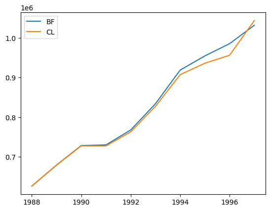
Let’s perform the estimate using Chainladder and compare the results.

bf_model.ultimate_.to_frame(origin_as_datetime=True).index.year

Index([1988, 1989, 1990, 1991, 1992, 1993, 1994, 1995, 1996, 1997], dtype='int32')

plt.plot(
    bf_model.ultimate_.to_frame(origin_as_datetime=True).index.year,
    bf_model.ultimate_.to_frame(origin_as_datetime=True),
    label="BF",
)

cl_model = cl.Chainladder().fit(comauto["CumPaidLoss"])
plt.plot(
    cl_model.ultimate_.to_frame(origin_as_datetime=True).index.year,
    cl_model.ultimate_.to_frame(origin_as_datetime=True),
    label="CL",
)

plt.legend(loc="upper left")

<matplotlib.legend.Legend at 0x7f9fdc2c6e50>

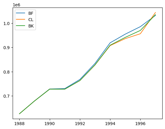
Benktander Method

The Benktander method is similar to the BornhuetterFerguson method, but allows for the specification of one additional assumption, n_iters, the number of iterations to recalculate the ultimates. The Benktander method generalizes both the BornhuetterFerguson and the Chainladder estimator through this assumption.

• When n_iters = 1, the result is equivalent to the BornhuetterFerguson estimator.

• When n_iters is sufficiently large, the result converges to the Chainladder estimator.

bk_model = cl.Benktander(apriori=0.75, n_iters=2)
bk_model.fit(
    comauto["CumPaidLoss"], sample_weight=comauto["EarnedPremNet"].latest_diagonal
)

Benktander(apriori=0.75, n_iters=2)

In a Jupyter environment, please rerun this cell to show the HTML representation or trust the notebook.
On GitHub, the HTML representation is unable to render, please try loading this page with nbviewer.org.

Fitting the Benktander method looks identical to the other methods.

bk_model.fit(
    X=comauto["CumPaidLoss"], sample_weight=comauto["EarnedPremNet"].latest_diagonal
)

Benktander(apriori=0.75, n_iters=2)

In a Jupyter environment, please rerun this cell to show the HTML representation or trust the notebook.
On GitHub, the HTML representation is unable to render, please try loading this page with nbviewer.org.

plt.plot(
    bf_model.ultimate_.to_frame(origin_as_datetime=True).index.year,
    bf_model.ultimate_.to_frame(origin_as_datetime=True),
    label="BF",
)
plt.plot(
    cl_model.ultimate_.to_frame(origin_as_datetime=True).index.year,
    cl_model.ultimate_.to_frame(origin_as_datetime=True),
    label="CL",
)
plt.plot(
    bk_model.ultimate_.to_frame(origin_as_datetime=True).index.year,
    bk_model.ultimate_.to_frame(origin_as_datetime=True),
    label="BK",
)
plt.legend(loc="upper left")

<matplotlib.legend.Legend at 0x7f9fdc1c2d90>

Cape Cod Method

The CapeCod method is similar to the BornhuetterFerguson method, except its apriori is computed from the Triangle itself. Instead of specifying an apriori, decay and trend need to be specified.

• decay is the rate that gives weights to earlier origin periods, this parameter is required by the Generalized Cape Cod Method, as discussed in Using Best Practices to Determine a Best Reserve Estimate by Struzzieri and Hussian. As the decay factor approaches 1 (the default value), the result approaches the traditional Cape Cod method. As the decay factor approaches 0, the result approaches the Chainladder method.

• trend is the trend rate along the origin axis to reflect systematic inflationary impacts on the a priori.

When we fit a CapeCod method, we can see the apriori it computes with the given decay and trend assumptions. Since it is an array of estimated parameters, this CapeCod attribute is called the apriori_, with a trailing underscore.

cc_model = cl.CapeCod()
cc_model.fit(
    comauto["CumPaidLoss"], sample_weight=comauto["EarnedPremNet"].latest_diagonal
)

CapeCod()

In a Jupyter environment, please rerun this cell to show the HTML representation or trust the notebook.
On GitHub, the HTML representation is unable to render, please try loading this page with nbviewer.org.

With decay=1, each origin period gets the same apriori_ (this is the traditional Cape Cod). The apriori_ is calculated using the latest diagonal over the used-up exposure, where the used-up exposure is the exposure vector / CDF. Let’s validate the calculation of the a priori.

latest_diagonal = comauto["CumPaidLoss"].latest_diagonal

cdf_as_origin_vector = (
    cl.Chainladder().fit(comauto["CumPaidLoss"]).ultimate_
    / comauto["CumPaidLoss"].latest_diagonal
)

latest_diagonal.sum() / (
    comauto["EarnedPremNet"].latest_diagonal / cdf_as_origin_vector
).sum()

0.6856862224535671

With decay=0, the apriori_ for each origin period stands on its own.

cc_model = cl.CapeCod(decay=0, trend=0).fit(
    X=comauto["CumPaidLoss"], sample_weight=comauto["EarnedPremNet"].latest_diagonal
)
cc_model.apriori_

	2261
1988	0.6853
1989	0.7041
1990	0.6903
1991	0.6478
1992	0.6518
1993	0.6815
1994	0.6925
1995	0.7004
1996	0.7039
1997	0.7619

Doing the same on our manually calculated apriori_ yields the same result.

latest_diagonal / (comauto["EarnedPremNet"].latest_diagonal / cdf_as_origin_vector)

	1997
1988	0.6853
1989	0.7041
1990	0.6903
1991	0.6478
1992	0.6518
1993	0.6815
1994	0.6925
1995	0.7004
1996	0.7039
1997	0.7619

Let’s verify the result of this Cape Cod model’s result with the Chainladder’s.

cc_model.ultimate_ - cl_model.ultimate_

	2261
1988
1989
1990
1991
1992	0.0000
1993	0.0000
1994
1995	0.0000
1996
1997	0.0000

We can examine the apriori_s to see whether there exhibit any trends over time.

plt.plot(
    cc_model.apriori_.to_frame(origin_as_datetime=True).index.year,
    cc_model.apriori_.to_frame(origin_as_datetime=True),
)

[<matplotlib.lines.Line2D at 0x7f9fdc0153d0>]

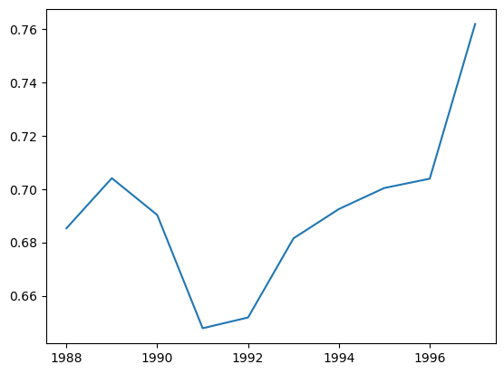
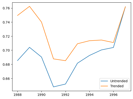
Looks like there is a small positive trend, let’s judgementally select the trend as 1%.

trended_cc_model = cl.CapeCod(decay=0, trend=0.01).fit(
    X=comauto["CumPaidLoss"], sample_weight=comauto["EarnedPremNet"].latest_diagonal
)

plt.plot(
    cc_model.apriori_.to_frame(origin_as_datetime=True).index.year,
    cc_model.apriori_.to_frame(origin_as_datetime=True),
    label="Untrended",
)
plt.plot(
    trended_cc_model.apriori_.to_frame(origin_as_datetime=True).index.year,
    trended_cc_model.apriori_.to_frame(origin_as_datetime=True),
    label="Trended",
)
plt.legend(loc="lower right")

<matplotlib.legend.Legend at 0x7f9fdc05b3d0>

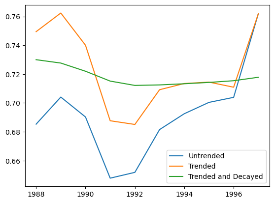
We can of course utilize both the trend and the decay parameters together. Adding trend to the CapeCod method is intended to adjust the apriori_s to a common level. Once at a common level, the apriori_ can be estimated from multiple origin periods using the decay factor.

trended_cc_model = cl.CapeCod(decay=0, trend=0.01).fit(
    X=comauto["CumPaidLoss"], sample_weight=comauto["EarnedPremNet"].latest_diagonal
)

trended_decayed_cc_model = cl.CapeCod(decay=0.75, trend=0.01).fit(
    X=comauto["CumPaidLoss"], sample_weight=comauto["EarnedPremNet"].latest_diagonal
)

plt.plot(
    cc_model.apriori_.to_frame(origin_as_datetime=True).index.year,
    cc_model.apriori_.to_frame(origin_as_datetime=True),
    label="Untrended",
)
plt.plot(
    trended_cc_model.apriori_.to_frame(origin_as_datetime=True).index.year,
    trended_cc_model.apriori_.to_frame(origin_as_datetime=True),
    label="Trended",
)
plt.plot(
    trended_decayed_cc_model.apriori_.to_frame(origin_as_datetime=True).index.year,
    trended_decayed_cc_model.apriori_.to_frame(origin_as_datetime=True),
    label="Trended and Decayed",
)
plt.legend(loc="lower right")

<matplotlib.legend.Legend at 0x7f9fdb7aad90>

Once estimated, it is necessary to detrend our apriori_s back to their untrended levels and these are contained in detrended_apriori_. It is the detrended_apriori_ that gets used in the calculation of ultimate_ losses.

plt.plot(
    trended_cc_model.apriori_.to_frame(origin_as_datetime=True).index.year,
    trended_cc_model.apriori_.to_frame(origin_as_datetime=True),
    label="Trended",
)
plt.plot(
    trended_cc_model.detrended_apriori_.to_frame(origin_as_datetime=True).index.year,
    trended_cc_model.detrended_apriori_.to_frame(origin_as_datetime=True),
    label="Detended to Original",
)
plt.legend(loc="lower right")

<matplotlib.legend.Legend at 0x7f9fdb663e50>

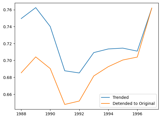
The detrended_apriori_ is a much smoother estimate of the initial expected ultimate_. With the detrended_apriori_ in hand, the CapeCod method estimator behaves exactly like our the BornhuetterFerguson model.

bf_model = cl.BornhuetterFerguson().fit(
    X=comauto["CumPaidLoss"],
    sample_weight=trended_cc_model.detrended_apriori_
    * comauto["EarnedPremNet"].latest_diagonal,
)

bf_model.ultimate_.sum() == trended_cc_model.ultimate_.sum()

True

Recap

All the deterministic estimators have ultimate_, ibnr_, full_expecation_ and full_triangle_ attributes that are themselves Triangles. These can be manipulated in a variety of ways to gain additional insights from our model. The expected loss methods take in an exposure vector, which itself is a Triangle through the sample_weight argument of the fit method. The CapeCod method has the additional attributes apriori_ and detrended_apriori_ to accommodate the selection of its trend and decay assumptions.

Finally, these estimators work very well with the transformers discussed in previous tutorials. Let’s demonstrate the compositional nature of these estimators.

wkcomp = (
    cl.load_sample("clrd")
    .groupby("LOB")
    .sum()
    .loc["wkcomp"][["CumPaidLoss", "EarnedPremNet"]]
)
wkcomp

	Triangle Summary
Valuation:	1997-12
Grain:	OYDY
Shape:	(1, 2, 10, 10)
Index:	[LOB]
Columns:	[CumPaidLoss, EarnedPremNet]

Let’s calculate the age-to-age factors:

• Without the the 1995 valuation period

• Using volume weighted for the first 5 factors, and simple average for the next 4 factors (for a total of 9 age-to-age factors)

• Using no more than 7 periods (with n_periods)

patterns = cl.Pipeline(
    [
        (
            "dev",
            cl.Development(
                average=["volume"] * 5 + ["simple"] * 4,
                n_periods=7,
                drop_valuation="1995",
            ),
        ),
        ("tail", cl.TailCurve(curve="inverse_power", extrap_periods=80)),
    ]
)

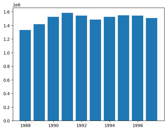
cc = cl.CapeCod(decay=0.8, trend=0.02).fit(
    X=patterns.fit_transform(wkcomp["CumPaidLoss"]),
    sample_weight=wkcomp["EarnedPremNet"].latest_diagonal,
)
cc.ultimate_

	2261
1988	1,331,221
1989	1,416,505
1990	1,523,470
1991	1,581,962
1992	1,541,458
1993	1,484,168
1994	1,525,963
1995	1,548,534
1996	1,541,068
1997	1,507,592

plt.bar(
    cc.ultimate_.to_frame(origin_as_datetime=True).index.year,
    cc.ultimate_.to_frame(origin_as_datetime=True)["2261"],
)

<BarContainer object of 10 artists>

Voting Chainladder

A VotingChainladder is an ensemble meta-estimator that fits several base chainladder methods, each on the whole triangle. Then it combines the individual predictions based on a matrix of weights to form a final prediction.

Let’s begin by loading the raa dataset.

raa = cl.load_sample("raa")

Instantiate the Chainladder’s estimator.

cl_mod = cl.Chainladder()

Instantiate the Expected Loss’s estimator.

el_mod = cl.ExpectedLoss(apriori=1)

Instantiate the Bornhuetter-Ferguson’s estimator. Remember that the BornhuetterFerguson requires one argument, the apriori.

bf_mod = cl.BornhuetterFerguson(apriori=1)

Instantiate the Cape Cod’s estimator and their required arguments.

cc_mod = cl.CapeCod(decay=1, trend=0)

Instantiate the Benktander’s estimator and their required arguments.

bk_mod = cl.Benktander(apriori=1, n_iters=2)

Let’s prepare the estimators variable. The estimators parameter in VotingChainladder must be in an array of tuples, with (estimator_name, estimator) pairing.

estimators = [
    ("cl", cl_mod),
    ("el", el_mod),
    ("bf", bf_mod),
    ("cc", cc_mod),
    ("bk", bk_mod),
]

Recall that some estimators (in this case, BornhuetterFerguson, CapeCod, and Benktander) also require the variable sample_weight, let’s use the mean of Chainladder’s average ultimate estimate.

sample_weight = cl_mod.fit(raa).ultimate_ * 0 + (
    float(cl_mod.fit(raa).ultimate_.sum()) / 10
)
sample_weight

	2261
1981	21,312
1982	21,312
1983	21,312
1984	21,312
1985	21,312
1986	21,312
1987	21,312
1988	21,312
1989	21,312
1990	21,312

model_weights = np.array(
    [[0.6, 0, 0.2, 0.2, 0]] * 4 + [[0, 0, 0.5, 0.5, 0]] * 3 + [[0, 0, 0, 1, 0]] * 3
)

vot_mod = cl.VotingChainladder(estimators=estimators, weights=model_weights).fit(
    raa, sample_weight=sample_weight
)
vot_mod.ultimate_

	2261
1981	18,834
1982	16,876
1983	24,059
1984	28,543
1985	28,237
1986	19,905
1987	18,947
1988	23,107
1989	20,005
1990	21,606

plt.plot(
    cl_mod.fit(raa).ultimate_.to_frame(origin_as_datetime=True).index.year,
    cl_mod.fit(raa).ultimate_.to_frame(origin_as_datetime=True),
    label="Chainladder",
    linestyle="dashed",
    marker="o",
)
plt.plot(
    el_mod.fit(raa, sample_weight=sample_weight)
    .ultimate_.to_frame(origin_as_datetime=True)
    .index.year,
    el_mod.fit(raa, sample_weight=sample_weight).ultimate_.to_frame(
        origin_as_datetime=True
    ),
    label="Expected Loss",
    linestyle="dashed",
    marker="o",
)
plt.plot(
    bf_mod.fit(raa, sample_weight=sample_weight)
    .ultimate_.to_frame(origin_as_datetime=True)
    .index.year,
    bf_mod.fit(raa, sample_weight=sample_weight).ultimate_.to_frame(
        origin_as_datetime=True
    ),
    label="Bornhuetter-Ferguson",
    linestyle="dashed",
    marker="o",
)
plt.plot(
    cc_mod.fit(raa, sample_weight=sample_weight)
    .ultimate_.to_frame(origin_as_datetime=True)
    .index.year,
    cc_mod.fit(raa, sample_weight=sample_weight).ultimate_.to_frame(
        origin_as_datetime=True
    ),
    label="Cape Cod",
    linestyle="dashed",
    marker="o",
)
plt.plot(
    bk_mod.fit(raa, sample_weight=sample_weight)
    .ultimate_.to_frame(origin_as_datetime=True)
    .index.year,
    bk_mod.fit(raa, sample_weight=sample_weight).ultimate_.to_frame(
        origin_as_datetime=True
    ),
    label="Benktander",
    linestyle="dashed",
    marker="o",
)
plt.plot(
    vot_mod.ultimate_.to_frame(origin_as_datetime=True).index.year,
    vot_mod.ultimate_.to_frame(origin_as_datetime=True),
    label="Selected",
)
plt.legend(loc="best")

<matplotlib.legend.Legend at 0x7f9fdb4dcd10>

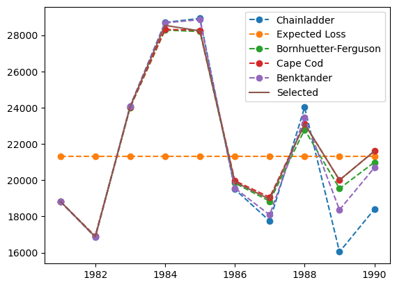
We can also call the weights attribute to confirm the weights being used by the VotingChainladder ensemble model.

vot_mod.weights

array([[0.6, 0. , 0.2, 0.2, 0. ],
       [0.6, 0. , 0.2, 0.2, 0. ],
       [0.6, 0. , 0.2, 0.2, 0. ],
       [0.6, 0. , 0.2, 0.2, 0. ],
       [0. , 0. , 0.5, 0.5, 0. ],
       [0. , 0. , 0.5, 0.5, 0. ],
       [0. , 0. , 0.5, 0.5, 0. ],
       [0. , 0. , 0. , 1. , 0. ],
       [0. , 0. , 0. , 1. , 0. ],
       [0. , 0. , 0. , 1. , 0. ]])