Applying Stochastic Methods#
Getting Started#
This tutorial focuses on using stochastic methods to estimate ultimates.
Be sure to make sure your packages are updated. For more info on how to update your pakages, visit Keeping Packages Updated.
# Black linter, optional
%load_ext lab_black

import pandas as pd
import numpy as np
import chainladder as cl
import matplotlib.pyplot as plt
import statsmodels.api as sm

print("pandas: " + pd.__version__)
print("numpy: " + np.__version__)
print("chainladder: " + cl.__version__)
pandas: 2.1.4
numpy: 1.24.3
chainladder: 0.8.18
Disclaimer#
Note that a lot of the examples shown might not be applicable in a real world scenario, and is only meant to demonstrate some of the functionalities included in the package. The user should always follow all applicable laws, the Code of Professional Conduct, applicable Actuarial Standards of Practice, and exercise their best actuarial judgement.
Intro to MackChainladder#
Like the basic Chainladder method, the MackChainladder is entirely specified by its selected development pattern. In fact, it is the basic Chainladder, but with extra features.
clrd = (
    cl.load_sample("clrd")
    .groupby("LOB")
    .sum()
    .loc["wkcomp", ["CumPaidLoss", "EarnedPremNet"]]
)

cl.Chainladder().fit(clrd["CumPaidLoss"]).ultimate_ == cl.MackChainladder().fit(
    clrd["CumPaidLoss"]
).ultimate_
True
Let’s create a Mack’s Chainladder model.
mack = cl.MackChainladder().fit(clrd["CumPaidLoss"])
MackChainladder has the following additional fitted features that the deterministic Chainladder does not:
full_std_err_: The full standard errortotal_process_risk_: The total process errortotal_parameter_risk_: The total parameter errormack_std_err_: The total prediction error by origin periodtotal_mack_std_err_: The total prediction error across all origin periods
Notice these are all measures of uncertainty, but where can they be applied? Let’s start by examining the link_ratios underlying the triangle between age 12 and 24.
clrd_first_lags = clrd[clrd.development <= 24][clrd.origin < "1997"]["CumPaidLoss"]
clrd_first_lags
| 12 | 24 | |
|---|---|---|
| 1988 | 285,804 | 638,532 |
| 1989 | 307,720 | 684,140 |
| 1990 | 320,124 | 757,479 |
| 1991 | 347,417 | 793,749 |
| 1992 | 342,982 | 781,402 |
| 1993 | 342,385 | 743,433 |
| 1994 | 351,060 | 750,392 |
| 1995 | 343,841 | 768,575 |
| 1996 | 381,484 | 736,040 |
A simple average link-ratio can be directly computed.
clrd_first_lags.link_ratio.to_frame(origin_as_datetime=True).mean()[0]
/tmp/ipykernel_3244/1055289506.py:1: FutureWarning: Series.__getitem__ treating keys as positions is deprecated. In a future version, integer keys will always be treated as labels (consistent with DataFrame behavior). To access a value by position, use `ser.iloc[pos]`
  clrd_first_lags.link_ratio.to_frame(origin_as_datetime=True).mean()[0]
2.2066789527531494
We can also verify that the result is the same as the Development object.
cl.Development(average="simple").fit(clrd["CumPaidLoss"]).ldf_.to_frame(
    origin_as_datetime=False
).values[0, 0]
2.2066789527531494
The Linear Regression Framework#
Mack noted that the estimate for the LDF is really just a linear regression fit. In the case of using the simple average, it is a weighted regression where the weight is $\left (\frac{1}{X} \right )^{2}$.
Let’s take a look at the fitted coefficient and verify that this ties to the direct calculations that we made earlier. With the regression framework in hand, we can get more information about our LDF estimate than just the coefficient.
y = clrd_first_lags.to_frame(origin_as_datetime=True).values[:, 1]
x = clrd_first_lags.to_frame(origin_as_datetime=True).values[:, 0]

model = sm.WLS(y, x, weights=(1 / x) ** 2)
results = model.fit()
results.summary()
/home/docs/checkouts/readthedocs.org/user_builds/chainladder-python/conda/latest/lib/python3.11/site-packages/scipy/stats/_stats_py.py:1806: UserWarning: kurtosistest only valid for n>=20 ... continuing anyway, n=9
  warnings.warn("kurtosistest only valid for n>=20 ... continuing "
| Dep. Variable: | y | R-squared (uncentered): | 0.997 |
|---|---|---|---|
| Model: | WLS | Adj. R-squared (uncentered): | 0.997 |
| Method: | Least Squares | F-statistic: | 2887. |
| Date: | Tue, 30 Jan 2024 | Prob (F-statistic): | 1.60e-11 |
| Time: | 16:29:27 | Log-Likelihood: | -107.89 |
| No. Observations: | 9 | AIC: | 217.8 |
| Df Residuals: | 8 | BIC: | 218.0 |
| Df Model: | 1 | ||
| Covariance Type: | nonrobust |
| coef | std err | t | P>|t| | [0.025 | 0.975] | |
|---|---|---|---|---|---|---|
| x1 | 2.2067 | 0.041 | 53.735 | 0.000 | 2.112 | 2.301 |
| Omnibus: | 7.448 | Durbin-Watson: | 1.177 |
|---|---|---|---|
| Prob(Omnibus): | 0.024 | Jarque-Bera (JB): | 2.533 |
| Skew: | -1.187 | Prob(JB): | 0.282 |
| Kurtosis: | 4.058 | Cond. No. | 1.00 |
Notes:
[1] R² is computed without centering (uncentered) since the model does not contain a constant.
[2] Standard Errors assume that the covariance matrix of the errors is correctly specified.
By toggling the weights of our regression, we can handle the most common types of averaging used in picking loss development factors.
For simple average, the weights are $\left (\frac{1}{X} \right )^{2}$
For volume-weighted average, the weights are $\left (\frac{1}{X} \right )$
For “regression” average, the weights are 1
print("Simple average:")
print(
    round(
        cl.Development(average="simple")
        .fit(clrd_first_lags)
        .ldf_.to_frame(origin_as_datetime=False)
        .values[0, 0],
        10,
    )
    == round(sm.WLS(y, x, weights=(1 / x) ** 2).fit().params[0], 10)
)

print("Volume-weighted average:")
print(
    round(
        cl.Development(average="volume")
        .fit(clrd_first_lags)
        .ldf_.to_frame(origin_as_datetime=False)
        .values[0, 0],
        10,
    )
    == round(sm.WLS(y, x, weights=(1 / x)).fit().params[0], 10)
)

print("Regression average:")
print(
    round(
        cl.Development(average="regression")
        .fit(clrd_first_lags)
        .ldf_.to_frame(origin_as_datetime=False)
        .values[0, 0],
        10,
    )
    == round(sm.OLS(y, x).fit().params[0], 10)
)
Simple average:
True
Volume-weighted average:
True
Regression average:
True
The regression framework is what the Development estimator uses to set development patterns. Although we discard the information in the deterministic methods, in the stochastic methods, Development has two useful statistics for estimating reserve variability, both of which come from the regression framework. The stastics are sigma_ and std_err_ , and they are used by the MackChainladder estimator to determine the prediction error of our reserves.
dev = cl.Development(average="simple").fit(clrd["CumPaidLoss"])
dev.sigma_
| 12-24 | 24-36 | 36-48 | 48-60 | 60-72 | 72-84 | 84-96 | 96-108 | 108-120 | |
|---|---|---|---|---|---|---|---|---|---|
| (All) | 0.1232 | 0.0340 | 0.0135 | 0.0091 | 0.0074 | 0.0067 | 0.0073 | 0.0097 | 0.0032 |
dev.std_err_
| 12-24 | 24-36 | 36-48 | 48-60 | 60-72 | 72-84 | 84-96 | 96-108 | 108-120 | |
|---|---|---|---|---|---|---|---|---|---|
| (All) | 0.0411 | 0.0120 | 0.0051 | 0.0037 | 0.0033 | 0.0033 | 0.0042 | 0.0068 | 0.0032 |
Remember that std_err_ is calculated as $\frac{\sigma}{\sqrt{N}}$.
np.round(
    dev.sigma_.to_frame(origin_as_datetime=False).transpose()["(All)"].values
    / np.sqrt(
        clrd["CumPaidLoss"].age_to_age.to_frame(origin_as_datetime=False).count()
    ).values,
    4,
)
array([0.0411, 0.012 , 0.0051, 0.0037, 0.0033, 0.0033, 0.0042, 0.0068,
       0.0032])
Since the regression framework uses the weighting method, we can easily turn “on and off” any observation we want using the dropping capabilities such as drop_valuation in the Development estimator. Dropping link ratios not only affects the ldf_ and cdf_, but also the std_err_ and sigma of the estimates.
Can we eliminate the 1988 valuation from our triangle, which is identical to eliminating the first observation from our 12-24 regression fit? Let’s calculate the std_err for the ldf_ of ages 12-24, and compare it to the value calculated using the weighted least squares regression.
clrd["CumPaidLoss"]
| 12 | 24 | 36 | 48 | 60 | 72 | 84 | 96 | 108 | 120 | |
|---|---|---|---|---|---|---|---|---|---|---|
| 1988 | 285,804 | 638,532 | 865,100 | 996,363 | 1,084,351 | 1,133,188 | 1,169,749 | 1,196,917 | 1,229,203 | 1,241,715 |
| 1989 | 307,720 | 684,140 | 916,996 | 1,065,674 | 1,154,072 | 1,210,479 | 1,249,886 | 1,291,512 | 1,308,706 | |
| 1990 | 320,124 | 757,479 | 1,017,144 | 1,169,014 | 1,258,975 | 1,315,368 | 1,368,374 | 1,394,675 | ||
| 1991 | 347,417 | 793,749 | 1,053,414 | 1,209,556 | 1,307,164 | 1,381,645 | 1,414,747 | |||
| 1992 | 342,982 | 781,402 | 1,014,982 | 1,172,915 | 1,281,864 | 1,328,801 | ||||
| 1993 | 342,385 | 743,433 | 959,147 | 1,113,314 | 1,187,581 | |||||
| 1994 | 351,060 | 750,392 | 993,751 | 1,114,842 | ||||||
| 1995 | 343,841 | 768,575 | 962,081 | |||||||
| 1996 | 381,484 | 736,040 | ||||||||
| 1997 | 340,132 |
round(
    cl.Development(average="volume", drop_valuation="1988")
    .fit(clrd["CumPaidLoss"])
    .std_err_.to_frame(origin_as_datetime=False)
    .values[0, 0],
    8,
) == round(sm.WLS(y[1:], x[1:], weights=(1 / x[1:])).fit().bse[0], 8)
True
With sigma_ and std_err_ in hand, Mack goes on to develop recursive formulas to estimate parameter_risk_ and process_risk_.
mack.parameter_risk_
| 12 | 24 | 36 | 48 | 60 | 72 | 84 | 96 | 108 | 120 | 9999 | |
|---|---|---|---|---|---|---|---|---|---|---|---|
| 1988 | 0 | 0 | 0 | 0 | 0 | 0 | 0 | 0 | 0 | 0 | 0 |
| 1989 | 0 | 0 | 0 | 0 | 0 | 0 | 0 | 0 | 0 | 5,251 | 5,251 |
| 1990 | 0 | 0 | 0 | 0 | 0 | 0 | 0 | 0 | 9,520 | 11,183 | 11,183 |
| 1991 | 0 | 0 | 0 | 0 | 0 | 0 | 0 | 5,984 | 11,629 | 13,161 | 13,161 |
| 1992 | 0 | 0 | 0 | 0 | 0 | 0 | 4,588 | 7,468 | 12,252 | 13,648 | 13,648 |
| 1993 | 0 | 0 | 0 | 0 | 0 | 4,037 | 5,981 | 8,187 | 12,259 | 13,502 | 13,502 |
| 1994 | 0 | 0 | 0 | 0 | 4,163 | 5,980 | 7,555 | 9,503 | 13,302 | 14,506 | 14,506 |
| 1995 | 0 | 0 | 0 | 4,921 | 6,736 | 8,137 | 9,446 | 11,118 | 14,502 | 15,620 | 15,620 |
| 1996 | 0 | 0 | 8,824 | 11,289 | 12,895 | 14,101 | 15,190 | 16,513 | 19,141 | 20,090 | 20,090 |
| 1997 | 0 | 14,499 | 21,075 | 24,749 | 27,093 | 28,657 | 29,907 | 31,164 | 33,103 | 33,897 | 33,897 |
mack.process_risk_
| 12 | 24 | 36 | 48 | 60 | 72 | 84 | 96 | 108 | 120 | 9999 | |
|---|---|---|---|---|---|---|---|---|---|---|---|
| 1988 | 0 | 0 | 0 | 0 | 0 | 0 | 0 | 0 | 0 | 0 | 0 |
| 1989 | 0 | 0 | 0 | 0 | 0 | 0 | 0 | 0 | 0 | 5,089 | 5,089 |
| 1990 | 0 | 0 | 0 | 0 | 0 | 0 | 0 | 0 | 12,716 | 13,898 | 13,898 |
| 1991 | 0 | 0 | 0 | 0 | 0 | 0 | 0 | 9,791 | 16,366 | 17,396 | 17,396 |
| 1992 | 0 | 0 | 0 | 0 | 0 | 0 | 8,935 | 13,298 | 18,626 | 19,555 | 19,555 |
| 1993 | 0 | 0 | 0 | 0 | 0 | 9,138 | 12,792 | 16,090 | 20,536 | 21,375 | 21,375 |
| 1994 | 0 | 0 | 0 | 0 | 10,225 | 14,116 | 16,973 | 19,773 | 23,695 | 24,492 | 24,492 |
| 1995 | 0 | 0 | 0 | 13,102 | 17,449 | 20,434 | 22,804 | 25,180 | 28,514 | 29,264 | 29,264 |
| 1996 | 0 | 0 | 25,020 | 31,626 | 35,692 | 38,468 | 40,646 | 42,711 | 45,298 | 46,052 | 46,052 |
| 1997 | 0 | 43,224 | 62,195 | 72,725 | 79,313 | 83,518 | 86,649 | 89,327 | 91,962 | 93,045 | 93,045 |
Assumption of Independence#
The Mack model makes a lot of assumptions about independence (i.e. the covariance between random processes is 0). This means that many of the Variance estimates in the MackChainladder model follow the form of $Var(A+B) = Var(A)+Var(B)$.
First, mack_std_err_2 $=$ parameter_risk_2 $+$ process_risk_2, the parameter risk and process risk is assumed to be independent.
mack.parameter_risk_**2 + mack.process_risk_**2
| 12 | 24 | 36 | 48 | 60 | 72 | 84 | 96 | 108 | 120 | 9999 | |
|---|---|---|---|---|---|---|---|---|---|---|---|
| 1988 | |||||||||||
| 1989 | 53,474,629 | 53,474,629 | |||||||||
| 1990 | 252,315,077 | 318,202,202 | 318,202,202 | ||||||||
| 1991 | 131,677,828 | 403,094,112 | 475,836,802 | 475,836,802 | |||||||
| 1992 | 100,880,179 | 232,603,431 | 497,040,939 | 568,692,440 | 568,692,440 | ||||||
| 1993 | 99,801,841 | 199,401,152 | 325,904,005 | 572,006,803 | 639,209,994 | 639,209,994 | |||||
| 1994 | 121,874,576 | 235,033,680 | 345,157,930 | 481,280,614 | 738,380,263 | 810,270,433 | 810,270,433 | ||||
| 1995 | 195,879,863 | 349,828,815 | 483,758,514 | 609,246,045 | 757,631,482 | 1,023,325,766 | 1,100,370,499 | 1,100,370,499 | |||
| 1996 | 703,858,058 | 1,127,626,904 | 1,440,168,352 | 1,678,591,828 | 1,882,843,800 | 2,096,883,925 | 2,418,319,374 | 2,524,434,510 | 2,524,434,510 | ||
| 1997 | 2,078,583,588 | 4,312,427,152 | 5,901,421,925 | 7,024,556,506 | 7,796,506,775 | 8,402,465,469 | 8,950,516,203 | 9,552,739,954 | 9,806,329,251 | 9,806,329,251 |
mack.mack_std_err_**2
| 12 | 24 | 36 | 48 | 60 | 72 | 84 | 96 | 108 | 120 | 9999 | |
|---|---|---|---|---|---|---|---|---|---|---|---|
| 1988 | 0 | 0 | 0 | 0 | 0 | 0 | 0 | 0 | 0 | 0 | 0 |
| 1989 | 0 | 0 | 0 | 0 | 0 | 0 | 0 | 0 | 0 | 53,474,629 | 53,474,629 |
| 1990 | 0 | 0 | 0 | 0 | 0 | 0 | 0 | 0 | 252,315,077 | 318,202,202 | 318,202,202 |
| 1991 | 0 | 0 | 0 | 0 | 0 | 0 | 0 | 131,677,828 | 403,094,112 | 475,836,802 | 475,836,802 |
| 1992 | 0 | 0 | 0 | 0 | 0 | 0 | 100,880,179 | 232,603,431 | 497,040,939 | 568,692,440 | 568,692,440 |
| 1993 | 0 | 0 | 0 | 0 | 0 | 99,801,841 | 199,401,152 | 325,904,005 | 572,006,803 | 639,209,994 | 639,209,994 |
| 1994 | 0 | 0 | 0 | 0 | 121,874,576 | 235,033,680 | 345,157,930 | 481,280,614 | 738,380,263 | 810,270,433 | 810,270,433 |
| 1995 | 0 | 0 | 0 | 195,879,863 | 349,828,815 | 483,758,514 | 609,246,045 | 757,631,482 | 1,023,325,766 | 1,100,370,499 | 1,100,370,499 |
| 1996 | 0 | 0 | 703,858,058 | 1,127,626,904 | 1,440,168,352 | 1,678,591,828 | 1,882,843,800 | 2,096,883,925 | 2,418,319,374 | 2,524,434,510 | 2,524,434,510 |
| 1997 | 0 | 2,078,583,588 | 4,312,427,152 | 5,901,421,925 | 7,024,556,506 | 7,796,506,775 | 8,402,465,469 | 8,950,516,203 | 9,552,739,954 | 9,806,329,251 | 9,806,329,251 |
Second, total_process_risk_ 2 $= \sum_{origin} $ process_risk_ 2, the process risk is assumed to be independent between origins.
mack.total_process_risk_**2
| 12 | 24 | 36 | 48 | 60 | 72 | 84 | 96 | 108 | 120 | 9999 | |
|---|---|---|---|---|---|---|---|---|---|---|---|
| 1988 | 0 | 1,868,353,581 | 4,494,250,661 | 6,460,788,043 | 7,973,402,703 | 9,155,354,146 | 10,211,709,420 | 11,360,087,730 | 13,081,563,688 | 13,595,400,487 | 13,595,400,487 |
(mack.process_risk_**2).sum(axis="origin")
| 12 | 24 | 36 | 48 | 60 | 72 | 84 | 96 | 108 | 120 | 9999 | |
|---|---|---|---|---|---|---|---|---|---|---|---|
| 1988 | 1,868,353,581 | 4,494,250,661 | 6,460,788,043 | 7,973,402,703 | 9,155,354,146 | 10,211,709,420 | 11,360,087,730 | 13,081,563,688 | 13,595,400,487 | 13,595,400,487 |
Lastly, independence is also assumed to apply to the overall standard error of reserves, as expected.
(mack.parameter_risk_**2 + mack.process_risk_**2).sum(axis=2).sum(axis=3)
106117274249.93411
(mack.mack_std_err_**2).sum(axis=2).sum(axis=3)
106117274249.93411
This over-reliance on independence is one of the weaknesses of the MackChainladder method. Nevertheless, if the data align with this assumption, then total_mack_std_err_ is a reasonable esimator of reserve variability.
Mack Reserve Variability#
The mack_std_err_ at ultimate is the reserve variability for each origin period.
mack.mack_std_err_[
    mack.mack_std_err_.development == mack.mack_std_err_.development.max()
]
| 9999 | |
|---|---|
| 1988 | |
| 1989 | 7,313 |
| 1990 | 17,838 |
| 1991 | 21,814 |
| 1992 | 23,847 |
| 1993 | 25,283 |
| 1994 | 28,465 |
| 1995 | 33,172 |
| 1996 | 50,244 |
| 1997 | 99,027 |
With the summary_ method, we can more easily look at the result of the MackChainladder model.
mack.summary_
| Latest | IBNR | Ultimate | Mack Std Err | |
|---|---|---|---|---|
| 1988 | 1,241,715 | 1,241,715 | ||
| 1989 | 1,308,706 | 13,321 | 1,322,027 | 7,313 |
| 1990 | 1,394,675 | 42,210 | 1,436,885 | 17,838 |
| 1991 | 1,414,747 | 79,409 | 1,494,156 | 21,814 |
| 1992 | 1,328,801 | 119,709 | 1,448,510 | 23,847 |
| 1993 | 1,187,581 | 167,192 | 1,354,773 | 25,283 |
| 1994 | 1,114,842 | 260,401 | 1,375,243 | 28,465 |
| 1995 | 962,081 | 402,403 | 1,364,484 | 33,172 |
| 1996 | 736,040 | 636,834 | 1,372,874 | 50,244 |
| 1997 | 340,132 | 1,056,335 | 1,396,467 | 99,027 |
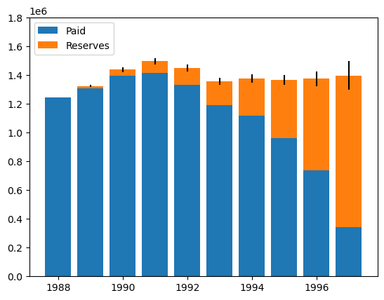
Let’s visualize the paid to date, the estimated reserves, and their standard errors with a histogram.
plt.bar(
    mack.summary_.to_frame(origin_as_datetime=True).index.year,
    mack.summary_.to_frame(origin_as_datetime=True)["Latest"],
    label="Paid",
)
plt.bar(
    mack.summary_.to_frame(origin_as_datetime=True).index.year,
    mack.summary_.to_frame(origin_as_datetime=True)["IBNR"],
    bottom=mack.summary_.to_frame(origin_as_datetime=True)["Latest"],
    yerr=mack.summary_.to_frame(origin_as_datetime=True)["Mack Std Err"],
    label="Reserves",
)
plt.legend(loc="upper left")
plt.ylim(0, 1800000)
(0.0, 1800000.0)
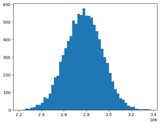
We can also simulate the (assumed) normally distributed IBNR with np.random.normal().
ibnr_mean = mack.ibnr_.sum()
ibnr_sd = mack.total_mack_std_err_.values[0, 0]
n_trials = 10000

np.random.seed(2021)
dist = np.random.normal(ibnr_mean, ibnr_sd, size=n_trials)

plt.hist(dist, bins=50)
(array([  1.,   2.,   8.,   7.,  13.,  17.,  30.,  29.,  41.,  72.,  66.,
         94., 142., 185., 195., 274., 312., 351., 392., 419., 509., 491.,
        546., 540., 577., 537., 534., 524., 483., 448., 401., 348., 300.,
        268., 210., 163., 118.,  94.,  68.,  59.,  41.,  25.,  19.,  18.,
          7.,   5.,   3.,   5.,   5.,   4.]),
 array([2209836.99059939, 2233093.4303693 , 2256349.87013921,
        2279606.30990912, 2302862.74967904, 2326119.18944895,
        2349375.62921886, 2372632.06898877, 2395888.50875869,
        2419144.9485286 , 2442401.38829851, 2465657.82806842,
        2488914.26783834, 2512170.70760825, 2535427.14737816,
        2558683.58714807, 2581940.02691799, 2605196.4666879 ,
        2628452.90645781, 2651709.34622773, 2674965.78599764,
        2698222.22576755, 2721478.66553746, 2744735.10530738,
        2767991.54507729, 2791247.9848472 , 2814504.42461711,
        2837760.86438702, 2861017.30415694, 2884273.74392685,
        2907530.18369676, 2930786.62346667, 2954043.06323659,
        2977299.5030065 , 3000555.94277641, 3023812.38254632,
        3047068.82231624, 3070325.26208615, 3093581.70185606,
        3116838.14162597, 3140094.58139589, 3163351.0211658 ,
        3186607.46093571, 3209863.90070562, 3233120.34047554,
        3256376.78024545, 3279633.22001536, 3302889.65978527,
        3326146.09955519, 3349402.5393251 , 3372658.97909501]),
 <BarContainer object of 50 artists>)
ODP Bootstrap Model#
The MackChainladder focuses on a regression framework for determining the variability of reserve estimates. An alternative approach is to use the statistical bootstrapping, or sampling from a triangle with replacement to simulate new triangles.
Bootstrapping imposes less model constraints than the MackChainladder, which allows for greater applicability in different scenarios. Sampling new triangles can be accomplished through the BootstrapODPSample estimator. This estimator will take a single triangle and simulate new ones from it. To simulate new triangles randomly from an existing triangle, we specify n_sims with how many triangles we want to simulate, and access the resampled_triangles_ attribute to get the simulated triangles. Notice that the shape of resampled_triangles_ matches n_sims at the first index.
samples = (
    cl.BootstrapODPSample(n_sims=10000).fit(clrd["CumPaidLoss"]).resampled_triangles_
)
samples
| Triangle Summary | |
|---|---|
| Valuation: | 1997-12 |
| Grain: | OYDY |
| Shape: | (10000, 1, 10, 10) |
| Index: | [LOB] |
| Columns: | [CumPaidLoss] |
Alternatively, we could use BootstrapODPSample to transform our triangle into a resampled set.
The notion of the ODP Bootstrap is that as our simulations approach infinity, we should expect our mean simulation to converge on the basic Chainladder estimate of of reserves.
Let’s apply the basic chainladder to our original triangle and also to our simulated triangles to see whether this holds true.
ibnr_cl = cl.Chainladder().fit(clrd["CumPaidLoss"]).ibnr_.sum()
ibnr_bootstrap = cl.Chainladder().fit(samples).ibnr_.sum("origin").mean()

print(
    "Chainladder's IBNR estimate:",
    ibnr_cl,
)
print(
    "BootstrapODPSample's mean IBNR estimate:",
    ibnr_bootstrap,
)
print("Difference $:", ibnr_cl - ibnr_bootstrap)
print("Difference %:", abs(ibnr_cl - ibnr_bootstrap) / ibnr_cl)
Chainladder's IBNR estimate: 2777812.6890986315
BootstrapODPSample's mean IBNR estimate: 2777494.70036822
Difference $: 317.9887304115109
Difference %: 0.00011447450422393118
Using Deterministic Methods with Bootstrapped Samples#
Our samples is just another triangle object with all the functionality of a regular triangle. This means we can apply any functionality we want to our samples including any deterministic methods we learned about previously.
pipe = cl.Pipeline(
    steps=[("dev", cl.Development(average="simple")), ("tail", cl.TailConstant(1.05))]
)

pipe.fit(samples)
Pipeline(steps=[('dev', Development(average='simple')),
                ('tail', TailConstant(tail=1.05))])
In a Jupyter environment, please rerun this cell to show the HTML representation or trust the notebook. On GitHub, the HTML representation is unable to render, please try loading this page with nbviewer.org.
Pipeline(steps=[('dev', Development(average='simple')),
('tail', TailConstant(tail=1.05))])Development(average='simple')
TailConstant(tail=1.05)
Now instead of a single ldf_ (and cdf_) array across developmental ages, we have 10,000 arrays of ldf_ (and cdf_).
pipe.named_steps.dev.ldf_.iloc[0]
| 12-24 | 24-36 | 36-48 | 48-60 | 60-72 | 72-84 | 84-96 | 96-108 | 108-120 | |
|---|---|---|---|---|---|---|---|---|---|
| (All) | 2.0994 | 1.3097 | 1.1561 | 1.0788 | 1.0479 | 1.0336 | 1.0205 | 1.0065 | 1.0108 |
pipe.named_steps.dev.ldf_.iloc[1]
| 12-24 | 24-36 | 36-48 | 48-60 | 60-72 | 72-84 | 84-96 | 96-108 | 108-120 | |
|---|---|---|---|---|---|---|---|---|---|
| (All) | 2.2037 | 1.3282 | 1.1488 | 1.0842 | 1.0441 | 1.0326 | 1.0252 | 1.0230 | 1.0133 |
pipe.named_steps.dev.ldf_.iloc[9999]
| 12-24 | 24-36 | 36-48 | 48-60 | 60-72 | 72-84 | 84-96 | 96-108 | 108-120 | |
|---|---|---|---|---|---|---|---|---|---|
| (All) | 2.2571 | 1.3184 | 1.1424 | 1.0802 | 1.0490 | 1.0287 | 1.0298 | 1.0202 | 1.0072 |
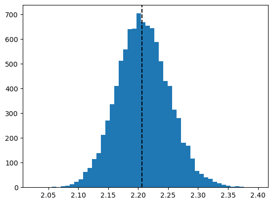
This allows us to look at the varibility of any fitted property used. Let’s look at the distribution of the age-to-age factor between age 12 and 24, and compare it against the LDF calculated from the non-bootstrapped triangle.
resampled_ldf = pipe.named_steps.dev.ldf_
plt.hist(pipe.named_steps.dev.ldf_.values[:, 0, 0, 0], bins=50)

orig_dev = cl.Development(average="simple").fit(clrd["CumPaidLoss"])
plt.axvline(orig_dev.ldf_.values[0, 0, 0, 0], color="black", linestyle="dashed")
<matplotlib.lines.Line2D at 0x7f3c200cbf10>
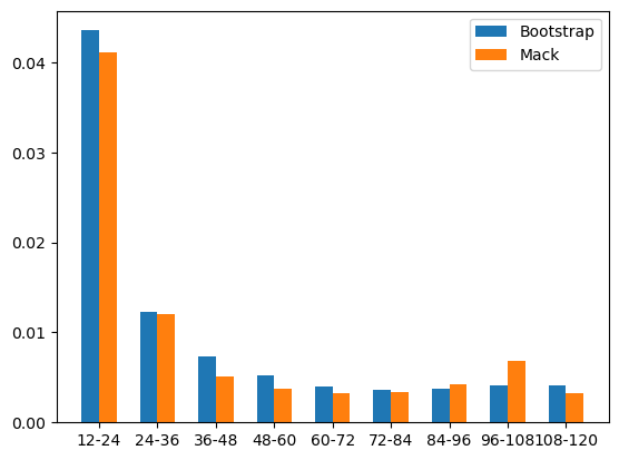
Bootstrap vs Mack#
We can approximate some of the Mack’s parameters calculated using the regression framework.
bootstrap_vs_mack = resampled_ldf.std("index").to_frame(origin_as_datetime=False).T
bootstrap_vs_mack.rename(columns={"(All)": "Std_Bootstrap"}, inplace=True)
bootstrap_vs_mack = bootstrap_vs_mack.merge(
    orig_dev.std_err_.to_frame(origin_as_datetime=False).T,
    left_index=True,
    right_index=True,
)
bootstrap_vs_mack.rename(columns={"(All)": "Std_Mack"}, inplace=True)

bootstrap_vs_mack
| Std_Bootstrap | Std_Mack | |
|---|---|---|
| 12-24 | 0.043550 | 0.041066 |
| 24-36 | 0.012341 | 0.012024 |
| 36-48 | 0.007317 | 0.005101 |
| 48-60 | 0.005264 | 0.003734 |
| 60-72 | 0.004043 | 0.003303 |
| 72-84 | 0.003679 | 0.003337 |
| 84-96 | 0.003723 | 0.004190 |
| 96-108 | 0.004093 | 0.006831 |
| 108-120 | 0.004150 | 0.003222 |
width = 0.3
ages = np.arange(len(bootstrap_vs_mack))

plt.bar(
    ages - width / 2,
    bootstrap_vs_mack["Std_Bootstrap"],
    width=width,
    label="Bootstrap",
)
plt.bar(ages + width / 2, bootstrap_vs_mack["Std_Mack"], width=width, label="Mack")
plt.legend(loc="upper right")
plt.xticks(ages, bootstrap_vs_mack.index)
([<matplotlib.axis.XTick at 0x7f3c201ce450>,
  <matplotlib.axis.XTick at 0x7f3c201cee90>,
  <matplotlib.axis.XTick at 0x7f3c20d56250>,
  <matplotlib.axis.XTick at 0x7f3c20221290>,
  <matplotlib.axis.XTick at 0x7f3c202234d0>,
  <matplotlib.axis.XTick at 0x7f3c20228bd0>,
  <matplotlib.axis.XTick at 0x7f3c2022afd0>,
  <matplotlib.axis.XTick at 0x7f3c20231150>,
  <matplotlib.axis.XTick at 0x7f3c20233310>],
 [Text(0, 0, '12-24'),
  Text(1, 0, '24-36'),
  Text(2, 0, '36-48'),
  Text(3, 0, '48-60'),
  Text(4, 0, '60-72'),
  Text(5, 0, '72-84'),
  Text(6, 0, '84-96'),
  Text(7, 0, '96-108'),
  Text(8, 0, '108-120')])
While the MackChainladder produces statistics about the mean and variance of reserve estimates, the variance or precentile of reserves would need to be fited using maximum likelihood estimation or method of moments. However, for BootstrapODPSample based fits, we can use the empirical distribution from the samples directly to get information about variance or the precentile of the IBNR reserves.
ibnr = cl.Chainladder().fit(samples).ibnr_.sum("origin")

ibnr_std = ibnr.std()
print("Standard deviation of reserve estimate: " + f"{round(ibnr_std,0):,}")
ibnr_99 = ibnr.quantile(q=0.99)
print("99th percentile of reserve estimate: " + f"{round(ibnr_99,0):,}")
Standard deviation of reserve estimate: 138,023.0
99th percentile of reserve estimate: 3,094,916.0
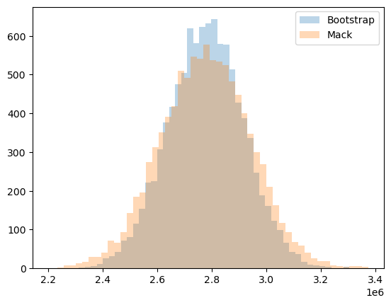
Let’s see how the MackChainladder reserve distribution compares to the BootstrapODPSample reserve distribution.
plt.hist(ibnr.to_frame(origin_as_datetime=True), bins=50, label="Bootstrap", alpha=0.3)
plt.hist(dist, bins=50, label="Mack", alpha=0.3)
plt.legend(loc="upper right")
<matplotlib.legend.Legend at 0x7f3c20267d10>
Expected Loss Methods with Bootstrap#
So far, we’ve only applied the multiplicative methods (i.e. basic chainladder) in a stochastic context. It is possible to use an expected loss method like the BornhuetterFerguson method does.
To do this, we will need an exposure vector.
sample_weight = clrd["EarnedPremNet"].latest_diagonal
Passing an apriori_sigma to the BornhuetterFerguson estimator tells it to consider the apriori selection itself as a random variable. Fitting a stochastic BornhuetterFerguson looks very much like the determinsitic version.
# Fit Bornhuetter-Ferguson to stochastically generated data
bf = cl.BornhuetterFerguson(0.65, apriori_sigma=0.10)
bf.fit(samples, sample_weight=sample_weight)
BornhuetterFerguson(apriori=0.65, apriori_sigma=0.1)In a Jupyter environment, please rerun this cell to show the HTML representation or trust the notebook.
On GitHub, the HTML representation is unable to render, please try loading this page with nbviewer.org.
BornhuetterFerguson(apriori=0.65, apriori_sigma=0.1)
We can use our knowledge of Triangle manipulation to grab most things we would want out of our model.
# Grab completed triangle replacing simulated known data with actual known data
full_triangle = bf.full_triangle_ - bf.X_ + clrd["CumPaidLoss"]
# Limiting to the current year for plotting
current_year = (
    full_triangle[full_triangle.origin == full_triangle.origin.max()]
    .to_frame(origin_as_datetime=True)
    .T
)
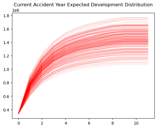
As expected, plotting the expected development of our full triangle over time from the Bootstrap BornhuetterFerguson model fans out to greater uncertainty the farther we get from our valuation date.
# Plot the data
current_year.iloc[:, :200].reset_index(drop=True).plot(
    color="red",
    legend=False,
    alpha=0.1,
    title="Current Accident Year Expected Development Distribution",
)
<Axes: title={'center': 'Current Accident Year Expected Development Distribution'}>
Recap#
The Mack method approaches stochastic reserving from a regression point of view
Bootstrap methods approach stochastic reserving from a simulation point of view
Where they assumptions of each model are not violated, they produce resonably consistent estimates of reserve variability
Mack does impose more assumptions (i.e. constraints) on the reserve estimate making the Bootstrap approach more suitable in a broader set of applciations
Both methods converge to their corresponding deterministic point estimates