PTF Residuals

import chainladder as cl
import pandas as pd

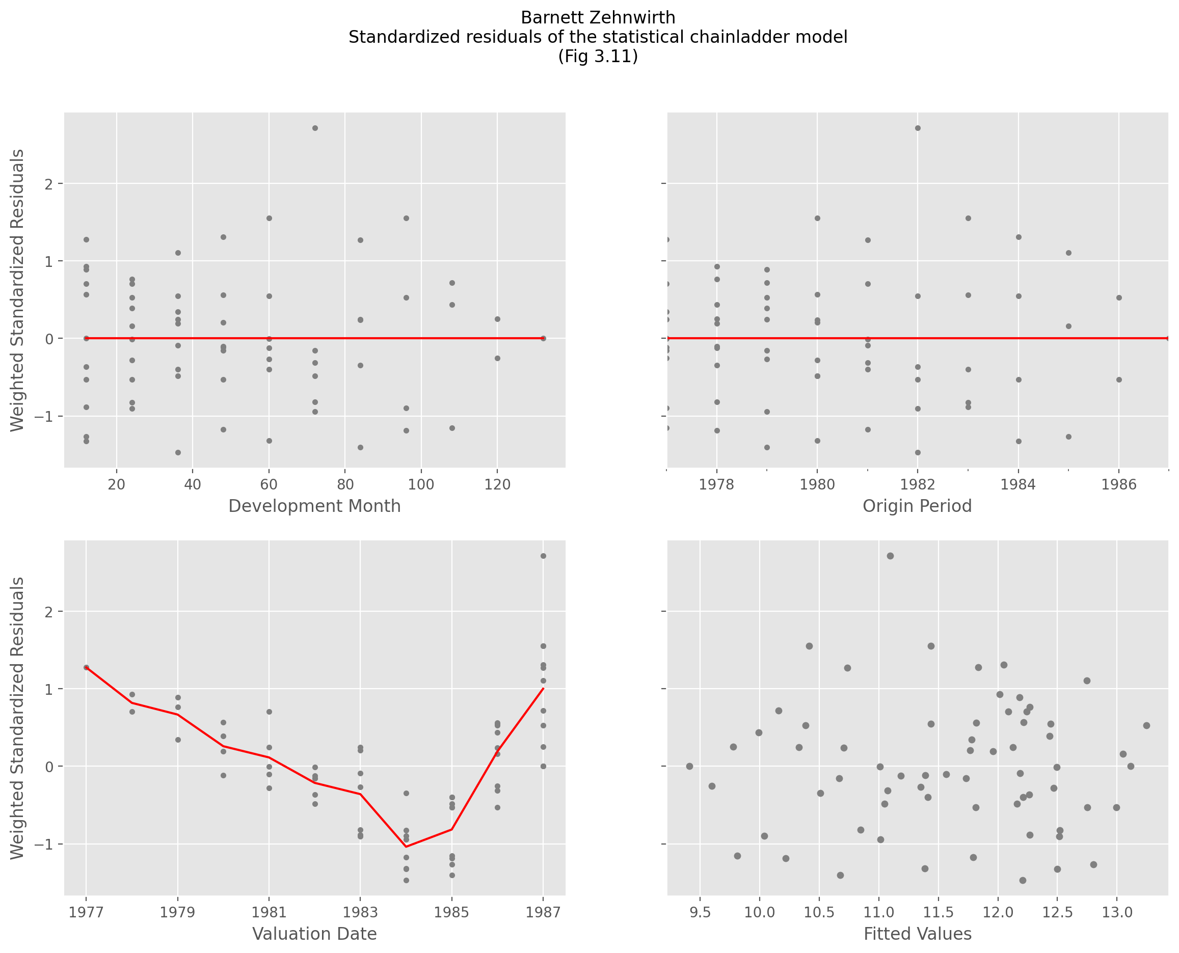
This example replicates the diagnostic residuals from Barnett and Zehnwirth’s “Best Estimates for Reserves” paper in which they describe the Probabilistic Trend Family (PTF) model. With the “ABC” triangle, they show that the basic chainladder, which ignores trend along the valuation axis, fails to have iid weighted standardized residuals along the valuation of the Triangle.

We fit a “diagnostic” model that deliberately ignores modeling the valuation vector. This is done by specifying the patsy formula C(origin)+C(development) which fits origin and development as categorical features.

abc = cl.load_sample('abc')
model = cl.BarnettZehnwirth(formula='C(origin) + C(development)').fit(abc)

plot1a = model.std_residuals_.T
plot1b = plot1a.T.mean()

plot2a = model.std_residuals_
plot2b = plot2a.T.mean()

plot3a = model.std_residuals_.dev_to_val().T
plot3b = model.std_residuals_.dev_to_val().mean('origin').T

plot4 = pd.concat((
    model.triangle_ml_[model.triangle_ml_.valuation<=abc.valuation_date].log().unstack().rename('Fitted Values'),
    model.std_residuals_.unstack().rename('Residual')), axis=1).dropna()

Show code cell source Hide code cell source

import matplotlib.pyplot as plt
plt.style.use('ggplot')
%config InlineBackend.figure_format = 'retina'

fig, ((ax00, ax01), (ax10, ax11)) = plt.subplots(ncols=2, nrows=2, figsize=(14,10))
fig.suptitle("Barnett Zehnwirth\nStandardized residuals of the statistical chainladder model\n(Fig 3.11)");

plot1a.plot(
    style='.', color='gray', legend=False, ax=ax00,
    xlabel='Development Month', ylabel='Weighted Standardized Residuals')
plot1b.plot(color='red', legend=False, ax=ax00)

plot2a.plot(style='.', color='gray', legend=False, ax=ax01, xlabel='Origin Period')
plot2b.plot(color='red', legend=False, ax=ax01)
plot3a.plot(
    style='.', color='gray', legend=False, ax=ax10,
    xlabel='Valuation Date', ylabel='Weighted Standardized Residuals')
plot3b.plot(color='red', legend=False, ax=ax10)

plot4.plot(kind='scatter', marker='o', color='gray', 
           x='Fitted Values', y='Residual', ax=ax11, sharey=True);