Data Preparation#
Getting Started#
This tutorial focuses on data, including a brief discussion on how to best prepare your data so it works well with the chainladder package.
Be sure to make sure your packages are updated. For more info on how to update your pakages, visit Keeping Packages Updated.
# Black linter, optional
%load_ext lab_black

import pandas as pd
import numpy as np
import chainladder as cl
import matplotlib.pyplot as plt

print("pandas: " + pd.__version__)
print("numpy: " + np.__version__)
print("chainladder: " + cl.__version__)
pandas: 2.1.4
numpy: 1.24.3
chainladder: 0.8.18
Disclaimer#
Note that a lot of the examples shown might not be applicable in a real world scenario, and is only meant to demonstrate some of the functionalities included in the package. The user should always follow all applicable laws, the Code of Professional Conduct, applicable Actuarial Standards of Practice, and exercise their best actuarial judgement.
Converting Triangle Data into Long Format#
One of the most commonly asked questions is that if the data needs to be in the tabular long format as opposed to the already processed triangle format when we are loading the data for use.
Unfortunately, the chainladder package requires the data to be in long form.
Suppose you have a wide triangle.
df = cl.load_sample("raa").to_frame(origin_as_datetime=True)
df
| 12 | 24 | 36 | 48 | 60 | 72 | 84 | 96 | 108 | 120 | |
|---|---|---|---|---|---|---|---|---|---|---|
| 1981-01-01 | 5012.0 | 8269.0 | 10907.0 | 11805.0 | 13539.0 | 16181.0 | 18009.0 | 18608.0 | 18662.0 | 18834.0 |
| 1982-01-01 | 106.0 | 4285.0 | 5396.0 | 10666.0 | 13782.0 | 15599.0 | 15496.0 | 16169.0 | 16704.0 | NaN |
| 1983-01-01 | 3410.0 | 8992.0 | 13873.0 | 16141.0 | 18735.0 | 22214.0 | 22863.0 | 23466.0 | NaN | NaN |
| 1984-01-01 | 5655.0 | 11555.0 | 15766.0 | 21266.0 | 23425.0 | 26083.0 | 27067.0 | NaN | NaN | NaN |
| 1985-01-01 | 1092.0 | 9565.0 | 15836.0 | 22169.0 | 25955.0 | 26180.0 | NaN | NaN | NaN | NaN |
| 1986-01-01 | 1513.0 | 6445.0 | 11702.0 | 12935.0 | 15852.0 | NaN | NaN | NaN | NaN | NaN |
| 1987-01-01 | 557.0 | 4020.0 | 10946.0 | 12314.0 | NaN | NaN | NaN | NaN | NaN | NaN |
| 1988-01-01 | 1351.0 | 6947.0 | 13112.0 | NaN | NaN | NaN | NaN | NaN | NaN | NaN |
| 1989-01-01 | 3133.0 | 5395.0 | NaN | NaN | NaN | NaN | NaN | NaN | NaN | NaN |
| 1990-01-01 | 2063.0 | NaN | NaN | NaN | NaN | NaN | NaN | NaN | NaN | NaN |
You can use pandas to unstack the data into the wide long format.
df = df.unstack().dropna().reset_index()
df.head(10)
| level_0 | level_1 | 0 | |
|---|---|---|---|
| 0 | 12 | 1981-01-01 | 5012.0 |
| 1 | 12 | 1982-01-01 | 106.0 |
| 2 | 12 | 1983-01-01 | 3410.0 |
| 3 | 12 | 1984-01-01 | 5655.0 |
| 4 | 12 | 1985-01-01 | 1092.0 |
| 5 | 12 | 1986-01-01 | 1513.0 |
| 6 | 12 | 1987-01-01 | 557.0 |
| 7 | 12 | 1988-01-01 | 1351.0 |
| 8 | 12 | 1989-01-01 | 3133.0 |
| 9 | 12 | 1990-01-01 | 2063.0 |
Let’s clean up our column names before we get too far.
df.columns = ["age", "origin", "values"]
df.head()
| age | origin | values | |
|---|---|---|---|
| 0 | 12 | 1981-01-01 | 5012.0 |
| 1 | 12 | 1982-01-01 | 106.0 |
| 2 | 12 | 1983-01-01 | 3410.0 |
| 3 | 12 | 1984-01-01 | 5655.0 |
| 4 | 12 | 1985-01-01 | 1092.0 |
Next, we will need a valuation column (think Schedule P style triangle).
df["valuation"] = (df["origin"].dt.year + df["age"] / 12 - 1).astype(int)
df.head()
| age | origin | values | valuation | |
|---|---|---|---|---|
| 0 | 12 | 1981-01-01 | 5012.0 | 1981 |
| 1 | 12 | 1982-01-01 | 106.0 | 1982 |
| 2 | 12 | 1983-01-01 | 3410.0 | 1983 |
| 3 | 12 | 1984-01-01 | 5655.0 | 1984 |
| 4 | 12 | 1985-01-01 | 1092.0 | 1985 |
Now, we are finally ready to load it into the chainladder package!
cl.Triangle(
    df, origin="origin", development="valuation", columns="values", cumulative=True
)
| 12 | 24 | 36 | 48 | 60 | 72 | 84 | 96 | 108 | 120 | |
|---|---|---|---|---|---|---|---|---|---|---|
| 1981 | 5,012 | 8,269 | 10,907 | 11,805 | 13,539 | 16,181 | 18,009 | 18,608 | 18,662 | 18,834 |
| 1982 | 106 | 4,285 | 5,396 | 10,666 | 13,782 | 15,599 | 15,496 | 16,169 | 16,704 | |
| 1983 | 3,410 | 8,992 | 13,873 | 16,141 | 18,735 | 22,214 | 22,863 | 23,466 | ||
| 1984 | 5,655 | 11,555 | 15,766 | 21,266 | 23,425 | 26,083 | 27,067 | |||
| 1985 | 1,092 | 9,565 | 15,836 | 22,169 | 25,955 | 26,180 | ||||
| 1986 | 1,513 | 6,445 | 11,702 | 12,935 | 15,852 | |||||
| 1987 | 557 | 4,020 | 10,946 | 12,314 | ||||||
| 1988 | 1,351 | 6,947 | 13,112 | |||||||
| 1989 | 3,133 | 5,395 | ||||||||
| 1990 | 2,063 |
Sparse Triangles#
By default, the chainladder Triangle is a wrapper around a numpy array. Numpy is optimized for high performance and this allows chainladder to achieve decent computational speeds. Despite being fast, numpy can become memory inefficient with triangle data because triangles are inherently sparse (when memory is being allocated yet no data is stored).
The lower half of a an incomplete triangle is generally blank and that means about 50% of an array size is wasted on empty space. As we include granular index and column values in our Triangle, the sparsity of the triangle increases further consuming RAM unnecessarily. Chainladder automatically eliminates this extraneous consumption of memory by resorting to a sparse array representation when the Triangle becomes sufficiently large.
Let’s load the prism dataset and include each claim number in the index of the Triangle. The dataset is claim level and includes over 130,000 triangles.
prism = cl.load_sample("prism")
prism
/home/docs/checkouts/readthedocs.org/user_builds/chainladder-python/conda/latest/lib/python3.11/site-packages/chainladder/core/base.py:250: UserWarning: The argument 'infer_datetime_format' is deprecated and will be removed in a future version. A strict version of it is now the default, see https://pandas.pydata.org/pdeps/0004-consistent-to-datetime-parsing.html. You can safely remove this argument.
  arr = dict(zip(datetime_arg, pd.to_datetime(**item)))
| Triangle Summary | |
|---|---|
| Valuation: | 2017-12 |
| Grain: | OMDM |
| Shape: | (34244, 4, 120, 120) |
| Index: | [ClaimNo, Line, Type, ClaimLiability, Limit, Deductible] |
| Columns: | [reportedCount, closedPaidCount, Paid, Incurred] |
Let’s also look at the array representation of the Triangle and notice how it is no longer a numpy array, but instead a sparse array.
prism.values
| Format | coo |
|---|---|
| Data Type | float64 |
| Shape | (34244, 4, 120, 120) |
| nnz | 121178 |
| Density | 6.143513381095148e-05 |
| Read-only | True |
| Size | 2.8M |
| Storage ratio | 0.00 |
The sparse array consumes about 4.6Mb of memory. We can also see its density is very low, this is because individual claims will at most exist in only one origin period. Let’s approximate the size of this Triangle assuming we used a dense array representation. Approximation can be done by assuming 8 bytes (for float64) of memory are used for each cell in the array.
print("Dense array size:", np.prod(prism.shape) / 1e6 * 8, "MB.")
print("Sparse array size:", prism.values.nbytes / 1e6, "MB.")
print(
    "Dense array is",
    round((np.prod(prism.shape) / 1e6 * 8) / (prism.values.nbytes / 1e6), 1),
    "times larger!",
)
Dense array size: 15779.6352 MB.
Sparse array size: 2.908272 MB.
Dense array is 5425.8 times larger!
Incremental vs Cumulative Triangles#
Cumulative triangles are naturally denser than those stored in an incremental fashion. While almost all actuarial techniques rely on cumulative triangles, it may be worthwhile to maintain and manipulate triangles as incremental triangles until you are ready to apply a model.
prism.values
| Format | coo |
|---|---|
| Data Type | float64 |
| Shape | (34244, 4, 120, 120) |
| nnz | 121178 |
| Density | 6.143513381095148e-05 |
| Read-only | True |
| Size | 2.8M |
| Storage ratio | 0.00 |
prism = prism.incr_to_cum()
prism.values
| Format | coo |
|---|---|
| Data Type | float64 |
| Shape | (34244, 4, 120, 120) |
| nnz | 5750047 |
| Density | 0.00291517360299939 |
| Read-only | True |
| Size | 219.3M |
| Storage ratio | 0.01 |
Our incremental triangle is under 5MB, but when we convert to a cumulative triangle it becomes an astonishingly large 219MB and this is despite still maintaining a sparsity of under 0.3%!
Claim-Level Data#
The sparse representation of triangles allows for substantially more data to be pushed through chainladder. This gives us some nice capabilities that we would not otherwise be able to do with aggregate data.
For example, we can now drill into the individual claim makeup of any cell in our Triangle. Let’s look at January 2017 claim details at age 12.
claims = prism[prism.origin == "2017-01"][prism.development == 12].to_frame(
    origin_as_datetime=True
)
claims[abs(claims).sum(axis="columns") != 0].reset_index()
| ClaimNo | Line | Type | ClaimLiability | Limit | Deductible | reportedCount | closedPaidCount | Paid | Incurred | |
|---|---|---|---|---|---|---|---|---|---|---|
| 0 | 38339 | Auto | PD | False | 8000.0 | 1000 | 1.0 | 0.0 | 0.000000 | 0.000000 |
| 1 | 38436 | Auto | PD | True | 15000.0 | 1000 | 1.0 | 1.0 | 8337.875863 | 8337.875863 |
| 2 | 38142 | Auto | PD | True | 8000.0 | 1000 | 1.0 | 1.0 | 7000.000000 | 7000.000000 |
| 3 | 38195 | Auto | PD | True | 20000.0 | 1000 | 1.0 | 1.0 | 19000.000000 | 19000.000000 |
| 4 | 38158 | Auto | PD | True | 20000.0 | 1000 | 1.0 | 1.0 | 10686.229420 | 10686.229420 |
| ... | ... | ... | ... | ... | ... | ... | ... | ... | ... | ... |
| 155 | 38393 | Auto | PD | True | 8000.0 | 1000 | 1.0 | 1.0 | 7000.000000 | 7000.000000 |
| 156 | 38396 | Auto | PD | True | 8000.0 | 1000 | 1.0 | 1.0 | 7000.000000 | 7000.000000 |
| 157 | 38455 | Auto | PD | True | 20000.0 | 1000 | 1.0 | 1.0 | 9927.351224 | 9927.351224 |
| 158 | 38457 | Auto | PD | True | 15000.0 | 1000 | 1.0 | 1.0 | 7874.879070 | 7874.879070 |
| 159 | 38460 | Auto | PD | True | 15000.0 | 1000 | 1.0 | 1.0 | 3125.840672 | 3125.840672 |
160 rows × 10 columns
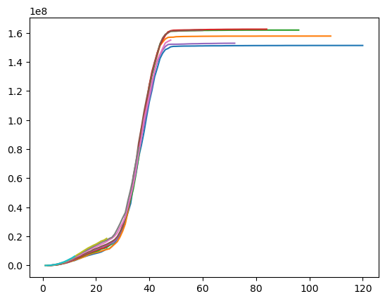
We can also examine the data as the usual aggregated Triangle, by applying sum(). We’ll also apply grain() so we can better visualize the data.
plt.plot(prism["Paid"].sum().grain("OYDM").to_frame(origin_as_datetime=True).T)
[<matplotlib.lines.Line2D at 0x7fce21a00f90>,
 <matplotlib.lines.Line2D at 0x7fce056cc8d0>,
 <matplotlib.lines.Line2D at 0x7fce056ce9d0>,
 <matplotlib.lines.Line2D at 0x7fce056cead0>,
 <matplotlib.lines.Line2D at 0x7fce056cf010>,
 <matplotlib.lines.Line2D at 0x7fce056cf490>,
 <matplotlib.lines.Line2D at 0x7fce056cf850>,
 <matplotlib.lines.Line2D at 0x7fce056cfc50>,
 <matplotlib.lines.Line2D at 0x7fce050b8050>,
 <matplotlib.lines.Line2D at 0x7fce056cf590>]
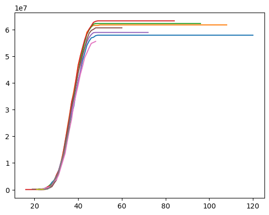
With claim level data, we can set a claim large loss cap or create an excess Triangle on the fly.
prism["Capped 100k Paid"] = cl.minimum(prism["Paid"], 100000)
prism["Excess 100k Paid"] = prism["Paid"] - prism["Capped 100k Paid"]
plt.plot(
    prism["Excess 100k Paid"].sum().grain("OYDM").to_frame(origin_as_datetime=True).T
)
[<matplotlib.lines.Line2D at 0x7fce2103a5d0>,
 <matplotlib.lines.Line2D at 0x7fce2103ab50>,
 <matplotlib.lines.Line2D at 0x7fce215ba9d0>,
 <matplotlib.lines.Line2D at 0x7fce2103a690>,
 <matplotlib.lines.Line2D at 0x7fce21039690>,
 <matplotlib.lines.Line2D at 0x7fce210380d0>,
 <matplotlib.lines.Line2D at 0x7fce210386d0>,
 <matplotlib.lines.Line2D at 0x7fce21038c50>,
 <matplotlib.lines.Line2D at 0x7fce21039210>,
 <matplotlib.lines.Line2D at 0x7fce2103a050>]
Claim-Level IBNR Estimates#
Let’s see how we can use the API to create claim-level IBNR estimates. When using aggregate actuarial techniques, it really makes sense to perform the model fitting at an aggregate level.
We use aggregate data to fit the model to generate reasonable development patterns.
agg_data = prism.sum()[["Paid", "reportedCount"]]
model_cl = cl.Chainladder().fit(agg_data)
With the fitted model, we are not limited to predicting ultimates at the aggregated grain. Let’s predict chainladder ultimates at a claim level. Here, we are using model_cl, which was built using agg_data to make prediction on prism, which is claim-level data.
cl_ults = model_cl.predict(prism[["Paid", "reportedCount"]]).ultimate_
cl_ults
| Triangle Summary | |
|---|---|
| Valuation: | 2261-12 |
| Grain: | OMDM |
| Shape: | (34244, 2, 120, 1) |
| Index: | [ClaimNo, Line, Type, ClaimLiability, Limit, Deductible] |
| Columns: | [Paid, reportedCount] |
We could stop here, but let’s try a Bornhuetter-Ferguson method as well. We will infer an a-priori severity from our chainladder model, model_cl above.
plt.plot(
    (model_cl.ultimate_["Paid"] / model_cl.ultimate_["reportedCount"]).to_frame(
        origin_as_datetime=True
    ),
)
[<matplotlib.lines.Line2D at 0x7fce21a1ac90>]
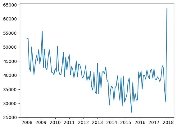
40K seems a reasonable a-priori (at least for the last two years or so, between 2016 - 2017).
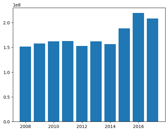
Now, let’s fit an aggregate Bornhuetter-Ferguson model. Like the chainladder example, we fit the model in aggregate (summing all claims) to create a stable model from which we can generate granular predictions. We will use our Chainladder ultimate claim counts as our sample_weight (exposure) for the BornhuetterFerguson method.
paid_bf = cl.BornhuetterFerguson(apriori=40000).fit(
    X=prism["Paid"].sum().incr_to_cum(), sample_weight=cl_ults["reportedCount"].sum()
)
plt.bar(
    paid_bf.ultimate_.grain("OYDM").to_frame(origin_as_datetime=False).index.year,
    paid_bf.ultimate_.grain("OYDM").to_frame(origin_as_datetime=False)["2261-12"],
)
<BarContainer object of 10 artists>
We can now create claim-level BornhuetterFerguson predictions using our claim-level Triangle. Ideally, the results should tie to the aggregate results.
bf_ults = paid_bf.predict(
    prism["Paid"].incr_to_cum(), sample_weight=cl_ults["reportedCount"]
).ultimate_
plt.bar(
    bf_ults.sum().grain("OYDM").to_frame(origin_as_datetime=False).index.year,
    bf_ults.sum().grain("OYDM").to_frame(origin_as_datetime=False)["2261-12"],
)
<BarContainer object of 10 artists>