BornhutterFerguson vs Chainladder

import chainladder as cl

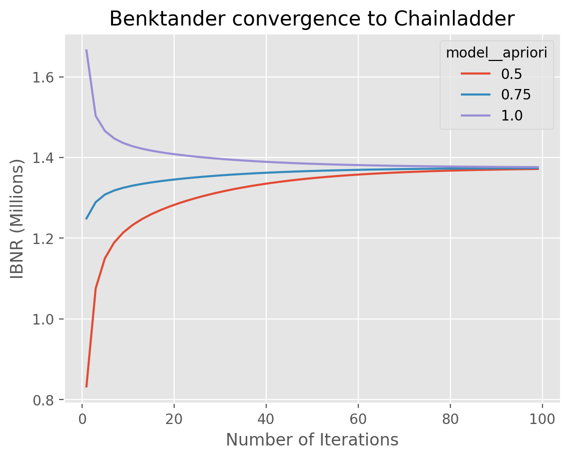
This example demonstrates the relationship between the Chainladder and BornhuetterFerguson methods by way of the Benktander model. Each is a special case of the Benktander model where n_iters = 1 for BornhuetterFerguson and as n_iters approaches infinity yields the chainladder. As n_iters increases the apriori selection becomes less relevant regardless of initial choice.

# Load Data
clrd = cl.load_sample('clrd').groupby('LOB').sum()
X = clrd.loc['medmal', 'CumPaidLoss']
sample_weight = clrd.loc['medmal', 'EarnedPremDIR'].latest_diagonal

# Specify Model
grid = cl.GridSearch(
    estimator=cl.Pipeline(steps=[
        ('dev', cl.Development()),
        ('tail', cl.TailCurve()),
        ('model', cl.Benktander())]), 
    param_grid = dict(
        model__n_iters=list(range(1, 100, 2)),
        model__apriori=[0.50, 0.75, 1.00]), 
    scoring={'IBNR': lambda x: x.named_steps.model.ibnr_.sum()},
    n_jobs=-1)

Because chainladder estimators are scikit-learn compatible, we can display them as expandable/collabsible diagrams.

from sklearn import set_config
set_config(display='diagram')
grid

GridSearch(estimator=Pipeline(steps=[('dev', Development()),
                                     ('tail', TailCurve()),
                                     ('model', Benktander())]),
           n_jobs=-1,
           param_grid={'model__apriori': [0.5, 0.75, 1.0],
                       'model__n_iters': [1, 3, 5, 7, 9, 11, 13, 15, 17, 19, 21,
                                          23, 25, 27, 29, 31, 33, 35, 37, 39,
                                          41, 43, 45, 47, 49, 51, 53, 55, 57,
                                          59, ...]},
           scoring={'IBNR': <function <lambda> at 0x7fe6d3964540>})

In a Jupyter environment, please rerun this cell to show the HTML representation or trust the notebook.
On GitHub, the HTML representation is unable to render, please try loading this page with nbviewer.org.

Fitting this model will loop through all param_grid options we specified and retain the aggregate IBNR of the model we declared in our scoring function.

# Fit Model
grid.fit(X, sample_weight=sample_weight)

# Analyze results
output = grid.results_.pivot(
    index='model__n_iters', 
    columns='model__apriori', 
    values='IBNR') 
output.head()

model__apriori	0.50	0.75	1.00
model__n_iters
1	8.326572e+05	1.248986e+06	1.665314e+06
3	1.075446e+06	1.289296e+06	1.503147e+06
5	1.150192e+06	1.308018e+06	1.465843e+06
7	1.189016e+06	1.318141e+06	1.447267e+06
9	1.214161e+06	1.324979e+06	1.435798e+06

Let’s plot the results of our output DataFrame.

Show code cell source Hide code cell source

import matplotlib.pyplot as plt
plt.style.use('ggplot')
%config InlineBackend.figure_format = 'retina'

ax = (output / 1e6).plot(
    ylabel='IBNR (Millions)',
    xlabel='Number of Iterations',
    title='Benktander convergence to Chainladder');