Triangle Creation Basics

import chainladder as cl
import pandas as pd

This example demonstrates the typical way you’d ingest data into a Triangle. Data in tabular form in a pandas DataFrame is required. At a minimum, columns specifying origin and development, and a value must be present. Note, you can include more than one column as a list as well as any number of indices for creating triangle subgroups.

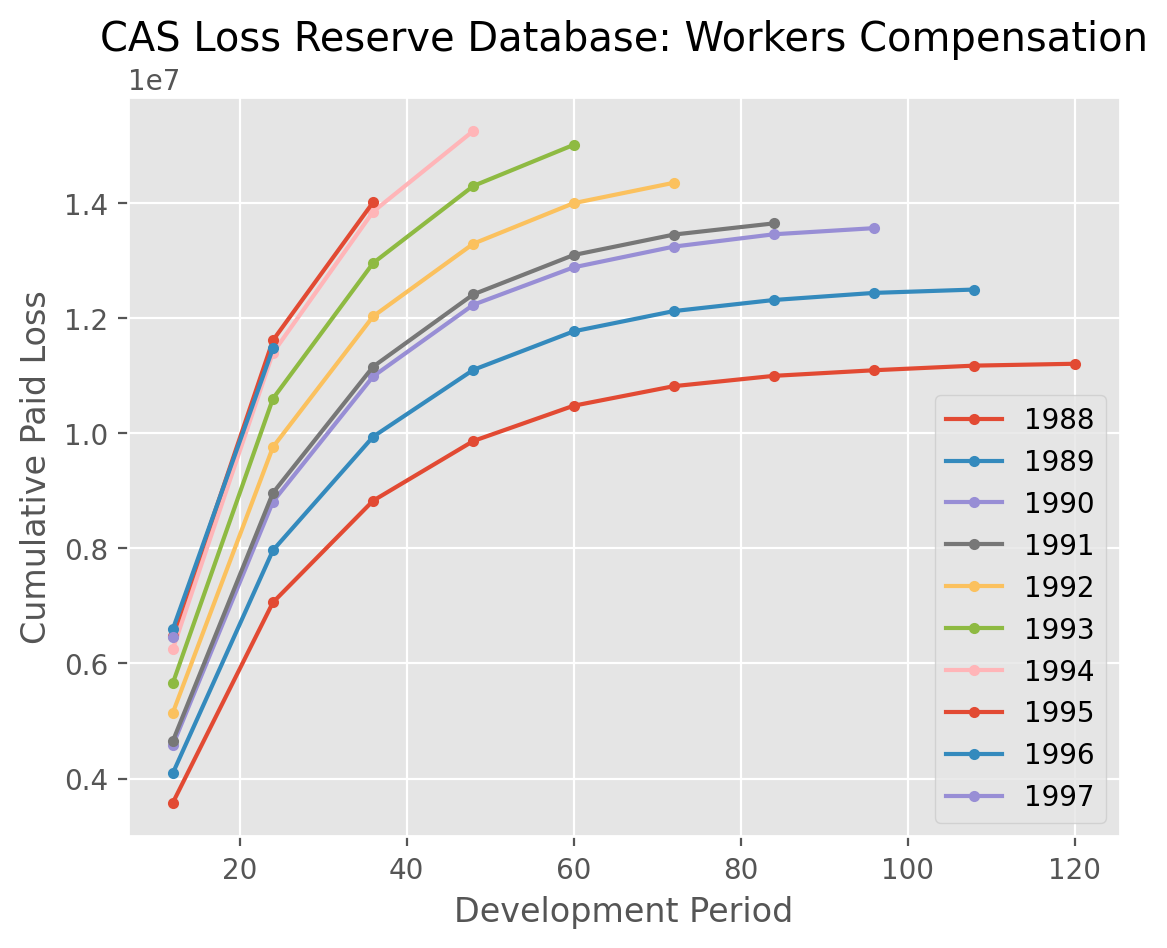
In this example, we create a triangle object with triangles for each company in the CAS Loss Reserve Database for Workers’ Compensation.

# Read in the data
data = pd.read_csv(r'https://raw.githubusercontent.com/casact/chainladder-python/master/chainladder/utils/data/clrd.csv')

# Output
data.head()

	GRCODE	GRNAME	AccidentYear	DevelopmentYear	DevelopmentLag	IncurLoss	CumPaidLoss	BulkLoss	EarnedPremDIR	EarnedPremCeded	EarnedPremNet	Single	PostedReserve97	LOB
0	86	Allstate Ins Co Grp	1988	1988	1	367404	70571	127737	400699	5957	394742	0	281872	wkcomp
1	86	Allstate Ins Co Grp	1988	1989	2	362988	155905	60173	400699	5957	394742	0	281872	wkcomp
2	86	Allstate Ins Co Grp	1988	1990	3	347288	220744	27763	400699	5957	394742	0	281872	wkcomp
3	86	Allstate Ins Co Grp	1988	1991	4	330648	251595	15280	400699	5957	394742	0	281872	wkcomp
4	86	Allstate Ins Co Grp	1988	1992	5	354690	274156	27689	400699	5957	394742	0	281872	wkcomp

# Create a triangle
triangle = cl.Triangle(
    data, origin='AccidentYear', development='DevelopmentYear',
    index=['GRNAME'], columns=['IncurLoss','CumPaidLoss','EarnedPremDIR'])

triangle

/home/docs/checkouts/readthedocs.org/user_builds/chainladder-python/conda/latest/lib/python3.11/site-packages/chainladder/core/triangle.py:189: UserWarning: 
            The cumulative property of your triangle is not set. This may result in
            undesirable behavior. In a future release this will result in an error.
  warnings.warn(

	Triangle Summary
Valuation:	1997-12
Grain:	OYDY
Shape:	(376, 3, 10, 10)
Index:	[GRNAME]
Columns:	[IncurLoss, CumPaidLoss, EarnedPremDIR]

triangle['CumPaidLoss'].sum()

	12	24	36	48	60	72	84	96	108	120
1988	3,577,780	7,059,966	8,826,151	9,862,687	10,474,698	10,814,576	10,994,014	11,091,363	11,171,590	11,203,949
1989	4,090,680	7,964,702	9,937,520	11,098,588	11,766,488	12,118,790	12,311,629	12,434,826	12,492,899
1990	4,578,442	8,808,486	10,985,347	12,229,001	12,878,545	13,238,667	13,452,993	13,559,557
1991	4,648,756	8,961,755	11,154,244	12,409,592	13,092,037	13,447,481	13,642,414
1992	5,139,142	9,757,699	12,027,983	13,289,485	13,992,821	14,347,271
1993	5,653,379	10,599,423	12,953,812	14,292,516	15,005,138
1994	6,246,447	11,394,960	13,845,764	15,249,326
1995	6,473,843	11,612,151	14,010,098
1996	6,591,599	11,473,912
1997	6,451,896

Show code cell source Hide code cell source

import matplotlib.pyplot as plt
plt.style.use('ggplot')
%config InlineBackend.figure_format = 'retina'

# Plot data
ax = triangle['CumPaidLoss'].sum().T.plot(
    marker='.', grid=True,
    title='CAS Loss Reserve Database: Workers Compensation',
    xlabel='Development Period', ylabel='Cumulative Paid Loss');