CapeCod Apriori Sensitivity#
import chainladder as cl
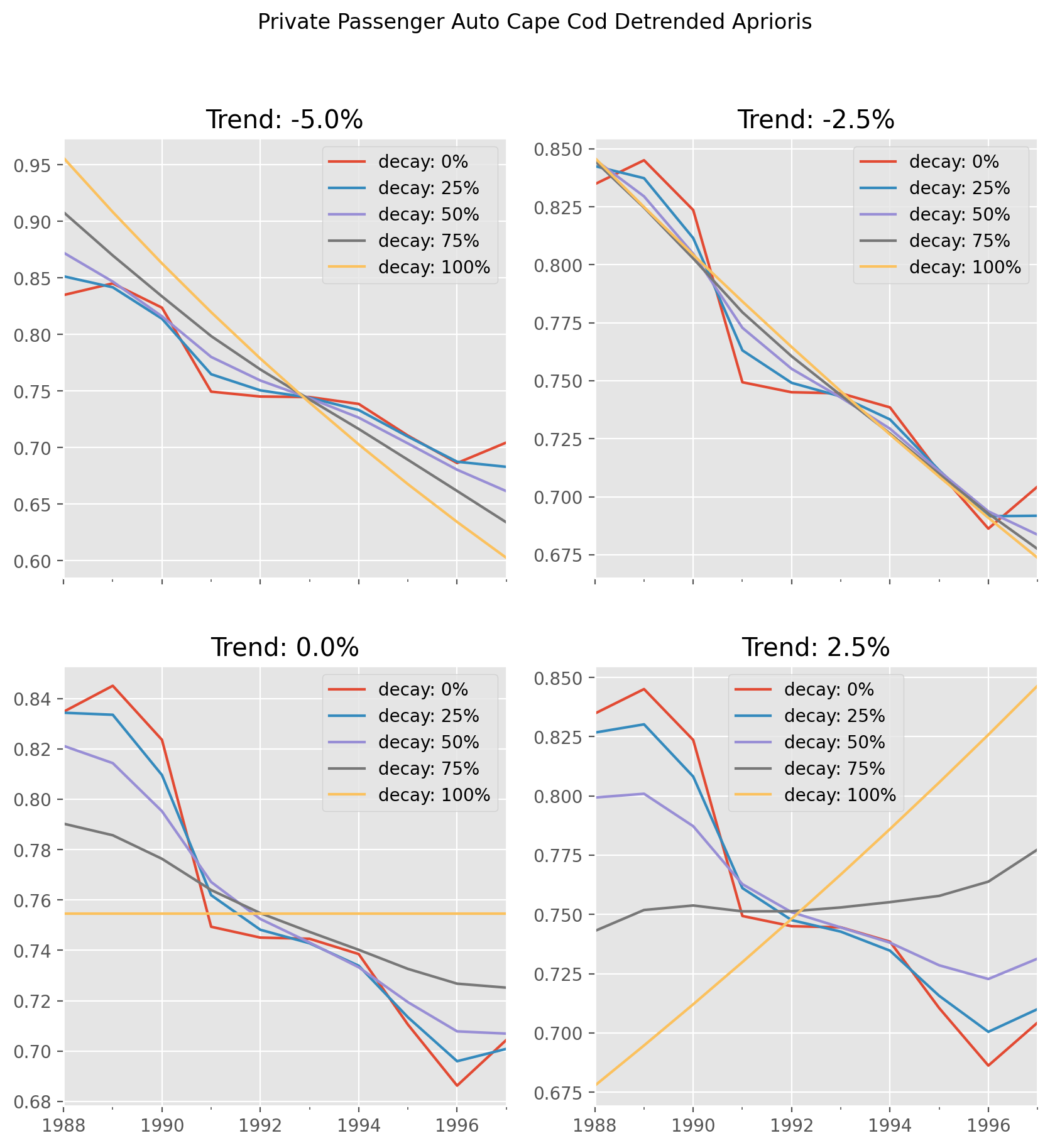
This example demonstrates the usage of the deterministic CapeCod method and
shows the sensitivity of the apriori expectation to various choices of trend
and decay. Instead of using GridSearch we declare our own looping.
# Grab data
ppauto_loss = cl.load_sample('clrd').groupby('LOB').sum().loc['ppauto', 'CumPaidLoss']
ppauto_prem = cl.load_sample('clrd').groupby('LOB').sum() \
                .loc['ppauto']['EarnedPremDIR'].latest_diagonal

def get_apriori(decay, trend):
    """ Function to grab apriori array from cape cod method """
    cc = cl.CapeCod(decay=decay, trend=trend)
    cc.fit(ppauto_loss, sample_weight=ppauto_prem)
    return cc.detrended_apriori_.to_frame()

def get_plot_data(trend):
    """ Function to grab plot data """
    # Initial apriori DataFrame
    detrended_aprioris = get_apriori(0,trend)
    detrended_aprioris.columns=['decay: 0%']

    # Add columns to apriori DataFrame
    for item in [25, 50, 75, 100]:
        detrended_aprioris[f'decay: {item}%'] = get_apriori(item/100, trend)
    return detrended_aprioris

# Plot Data
plot1 = get_plot_data(-0.05)
plot2 = get_plot_data(-.025)
plot3 = get_plot_data(0)
plot4 = get_plot_data(0.025)
import matplotlib.pyplot as plt
plt.style.use('ggplot')
%config InlineBackend.figure_format = 'retina'

fig, ((ax00, ax01), (ax10, ax11)) = plt.subplots(
    ncols=2, nrows=2, sharex=True, figsize=(10,10))
fig.suptitle("Private Passenger Auto Cape Cod Detrended Aprioris")
plot1.plot(ax=ax00, title='Trend: -5.0%')
plot2.plot(ax=ax01, title='Trend: -2.5%')
plot3.plot(ax=ax10, title='Trend: 0.0%')
plot4.plot(ax=ax11, title='Trend: 2.5%');