Workflow

Workflow#

chainladder facilitates practical reserving workflows.

import chainladder as cl
import numpy as np

import matplotlib.pyplot as plt
plt.style.use('ggplot')
%config InlineBackend.figure_format = 'retina'

Pipeline#

The :class:Pipeline class implements utilities to build a composite estimator, as a chain of transforms and estimators. Said differently, a Pipeline is a way to wrap multiple estimators into a single compact object. The Pipeline is borrowed from scikit-learn. As an example of compactness, we can simulate a set of triangles using bootstrap sampling, apply volume-weigted development, exponential tail curve fitting, and get the 95%-ile IBNR estimate.

pipe = cl.Pipeline(
    steps=[
    ('sample', cl.BootstrapODPSample(random_state=42)),
    ('dev', cl.Development(average='volume')),
    ('tail', cl.TailCurve('exponential')),
    ('model', cl.Chainladder())])

pipe.fit(cl.load_sample('genins'))

/home/docs/checkouts/readthedocs.org/user_builds/chainladder-python/envs/experimental/lib/python3.11/site-packages/chainladder/adjustments/bootstrap.py:284: UserWarning: 'where' used without 'out', expect unitialized memory in output. If this is intentional, use out=None.
  hat = xp.diagonal(xp.sqrt(xp.divide(1, abs(1 - hat), where=(1 - hat) != 0)))

Pipeline(steps=[('sample', BootstrapODPSample(random_state=42)),
                ('dev', Development()), ('tail', TailCurve()),
                ('model', Chainladder())])

In a Jupyter environment, please rerun this cell to show the HTML representation or trust the notebook.
On GitHub, the HTML representation is unable to render, please try loading this page with nbviewer.org.

Pipeline

iFitted

Parameters

	steps	[('sample', ...), ('dev', ...), ...]
	transform_input	None
	memory	None
	verbose	False

BootstrapODPSample

Parameters

	random_state	42
	n_sims	1000
	n_periods	-1
	hat_adj	True
	drop	None
	drop_high	None
	drop_low	None
	drop_valuation	None

Fitted attributes

Name	Type	Value
design_matrix_	ndarray[float64](55, 19)	[[1.,0.,0.,...,0.,0.,0.], [0.,1.,0.,...,0.,0.,0.], [0.,0.,1.,...,0.,0.,0.], ..., [1.,0.,0.,...,1.,1.,0.], [0.,1.,0.,...,1.,1.,0.], [1.,0.,0.,...,1.,1.,1.]]
hat_	ndarray[float64](10, 10)	[[1.09,1.16,1.17,...,1.2 ,1.36,0. ], [1.11,1.19,1.2 ,...,1.29,1.6 , nan], [1.11,1.19,1.21,...,1.29, nan, nan], ..., [1.18,1.41,1.44,..., nan, nan, nan], [1.26,1.99, nan,..., nan, nan, nan], [0. , nan, nan,..., nan, nan, nan]]
resampled_triangles_	Triangle	... [values]
scale_	float64	5.26e+04
w_	ndarray[float64](1, 1, 10, 9)	[[[[ 1., 1., 1.,..., 1., 1., 1.], [ 1., 1., 1.,..., 1., 1., 1.], [ 1., 1., 1.,..., 1., 1.,nan], ..., [ 1., 1., 1.,...,nan,nan,nan], [ 1., 1.,nan,...,nan,nan,nan], [ 1.,nan,nan,...,nan,nan,nan]]]]

Development

Parameters

	n_periods	-1
	average	'volume'
	sigma_interpolation	'log-linear'
	drop	None
	drop_high	None
	drop_low	None
	preserve	1
	drop_valuation	None
	drop_above	inf
	drop_below	0.0
	fillna	None
	groupby	None

Fitted attributes

Name	Type	Value
average_	ndarray[<U6](9,)	['volume','volume','volume',...,'volume','volume','volume']
cdf_	Triangle	Tr... [values]
ldf_	Triangle	Tr... [values]
sigma_	Triangle	Tr... [values]
std_err_	Triangle	Tr... [values]
std_residuals_	Triangle	Tr... [values]
w_	ndarray[float64](1000, 1, 10, 9)	[[[[ 1., 1., 1.,..., 1., 1., 1.], [ 1., 1., 1.,..., 1., 1., 1.], [ 1., 1., 1.,..., 1., 1.,nan], ..., [ 1., 1., 1.,...,nan,nan,nan], [ 1., 1.,nan,...,nan,nan,nan], [ 1.,nan,nan,...,nan,nan,nan]]], [[[ 1., 1., 1.,..., 1., 1., 1.], [ 1., 1., 1.,..., 1., 1., 1.], [ 1., 1., 1.,..., 1., 1.,nan], ..., [ 1., 1., 1.,...,nan,nan,nan], [ 1., 1.,nan,...,nan,nan,nan], [ 1.,nan,nan,...,nan,nan,nan]]], [[[ 1., 1., 1.,..., 1., 1., 1.], [ 1., 1., 1.,..., 1., 1., 1.], [ 1., 1., 1.,..., 1., 1.,nan], ..., [ 1., 1., 1.,...,nan,nan,nan], [ 1., 1.,nan,...,nan,nan,nan], [ 1.,nan,nan,...,nan,nan,nan]]], ..., [[[ 1., 1., 1.,..., 1., 1., 1.], [ 1., 1., 1.,..., 1., 1., 1.], [ 1., 1., 1.,..., 1., 1.,nan], ..., [ 1., 1., 1.,...,nan,nan,nan], [ 1., 1.,nan,...,nan,nan,nan], [ 1.,nan,nan,...,nan,nan,nan]]], [[[ 1., 1., 1.,..., 1., 1., 1.], [ 1., 1., 1.,..., 1., 1., 1.], [ 1., 1., 1.,..., 1., 1.,nan], ..., [ 1., 1., 1.,...,nan,nan,nan], [ 1., 1.,nan,...,nan,nan,nan], [ 1.,nan,nan,...,nan,nan,nan]]], [[[ 1., 1., 1.,..., 1., 1., 1.], [ 1., 1., 1.,..., 1., 1., 1.], [ 1., 1., 1.,..., 1., 1.,nan], ..., [ 1., 1., 1.,...,nan,nan,nan], [ 1., 1.,nan,...,nan,nan,nan], [ 1.,nan,nan,...,nan,nan,nan]]]]
w_v2_	Triangle	Tr... [values]

TailCurve

Parameters

	curve	'exponential'
	fit_period	(None, ...)
	extrap_periods	100
	errors	'ignore'
	attachment_age	None
	reg_threshold	(1.00001, ...)
	projection_period	12

Fitted attributes

Name	Type	Value
average_	ndarray[<U6](9,)	['volume','volume','volume',...,'volume','volume','volume']
cdf_	Triangle	T... [values]
intercept_	DataFrame	valu...s x 1 columns]
ldf_	Triangle	T... [values]
sigma_	Triangle	T... [values]
slope_	DataFrame	valu...s x 1 columns]
std_err_	Triangle	T... [values]
tail_	Series[float64](1000,)	Total 0 ...dtype: float64

Chainladder

Parameters

Fitted attributes

Name	Type	Value
X_	Triangle	... [values]
cdf_	Triangle	T... [values]
full_expectation_	Triangle	... [values]
full_triangle_	Triangle	... [values]
ibnr_	Triangle	T... [values]
ldf_	Triangle	T... [values]
process_variance_	Triangle	... [values]
sample_weight_	NoneType	None
ultimate_	Triangle	T... [values]

Each estimator contained within a pipelines steps can be accessed by name using the named_steps attribute of the Pipeline.

pipe.named_steps.model.ibnr_.sum('origin').quantile(q=.95)

np.float64(26063265.86634833)

As mentioned in the Development section, a Pipeline coupled with groupby can really streamline you reserving analysis. Here we can develop IBNR for each company using LOB level development patterns. By delegating the groupby operation to the Development estimator in the Pipeline, we can fully specify the entire analysis as part of our hyperparameters. This achieves a clear separation of assumption setting from data manipulation.

clrd = cl.load_sample('clrd')['CumPaidLoss']

pipe = cl.Pipeline(
    steps=[
    ('dev', cl.Development(groupby='LOB')),
    ('tail', cl.TailCurve('exponential')),
    ('model', cl.Chainladder())]).fit(clrd)

pipe.named_steps.model.ibnr_

	Triangle Summary
Valuation:	2261-12
Grain:	OYDY
Shape:	(775, 1, 10, 1)
Index:	[GRNAME, LOB]
Columns:	[CumPaidLoss]

VotingChainladder#

The :class:VotingChainladder ensemble method allows the actuary to vote between different underlying ibnr_ by way of a matrix of weights.

For example, the actuary may choose

the :class:Chainladder method for the first 4 origin periods,
the :class:BornhuetterFerguson method for the next 3 origin periods,
and the :class:CapeCod method for the final 3.

raa = cl.load_sample('RAA')
cl_ult = cl.Chainladder().fit(raa).ultimate_ # Chainladder Ultimate
apriori = cl_ult*0+(cl_ult.sum()/10) # Mean Chainladder Ultimate

bcl = cl.Chainladder()
bf = cl.BornhuetterFerguson()
cc = cl.CapeCod()

estimators = [('bcl', bcl), ('bf', bf), ('cc', cc)]
weights = np.array([[1, 0, 0]] * 4 + [[0, 1, 0]] * 3 + [[0, 0, 1]] * 3)
vot = cl.VotingChainladder(estimators=estimators, weights=weights)
vot.fit(raa, sample_weight=apriori)
vot.ultimate_

	2261
1981	18,834
1982	16,858
1983	24,083
1984	28,703
1985	28,204
1986	19,840
1987	18,840
1988	23,107
1989	20,005
1990	21,606

Alternatively, the actuary may choose to combine all methods using weights. Omitting the weights parameter results in the average of all predictions assuming a weight of 1. Alternatively, a default weight can be enforced through the default_weight parameter.

raa = cl.load_sample('RAA')
cl_ult = cl.Chainladder().fit(raa).ultimate_ # Chainladder Ultimate
apriori = cl_ult * 0 + (float(cl_ult.sum()) / 10) # Mean Chainladder Ultimate

bcl = cl.Chainladder()
bf = cl.BornhuetterFerguson()
cc = cl.CapeCod()

estimators = [('bcl', bcl), ('bf', bf), ('cc', cc)]
vot = cl.VotingChainladder(estimators=estimators)
vot.fit(raa, sample_weight=apriori)
vot.ultimate_

	2261
1981	18,834
1982	16,887
1983	24,042
1984	28,436
1985	28,467
1986	19,771
1987	18,548
1988	23,305
1989	18,530
1990	20,331

The weights can take the form of an array (as above), a dict, or a callable:

callable_weight = lambda origin : np.where(origin.year < 1985, (1, 0, 0), np.where(origin.year > 1987, (0, 0, 1), (0, 1, 0)))

dict_weight = {
    '1992': (0, 1, 0),
    '1993': (0, 1, 0),
    '1994': (0, 1, 0),
    '1995': (0, 0, 1),
    '1996': (0, 0, 1),
    '1997': (0, 0, 1),
}  # Unmapped origins will get `default_weight`

GridSearch#

The grid search provided by :class:GridSearch exhaustively generates candidates from a grid of parameter values specified with the param_grid parameter. Like Pipeline, GridSearch borrows from its scikit-learn counterpart GridSearchCV.

Because reserving techniques are different from supervised machine learning, GridSearch does not try to pick optimal hyperparameters for you. It is more of a scenario-testing estimator.

Tip

The tryangle package takes the machine learning aspect a bit farther than chainladder and has built in scoring functions that make hyperparameter tuning in a reserving context possible.

GridSearch can be applied to all other estimators, including the Pipeline estimator. To use it, one must specify a param_grid as well as a scoring function which defines the estimator property(s) you wish to capture.

pipe = cl.Pipeline(
    steps=[('dev', cl.Development()),
           ('model', cl.Chainladder())])

grid = cl.GridSearch(
    estimator=pipe,
    param_grid={'dev__average' :['volume', 'simple', 'regression']},
    scoring=lambda x : x.named_steps.model.ibnr_.sum('origin'))

grid.fit(cl.load_sample('genins'))
ax = grid.results_.set_index('dev__average').rename(columns={'score': 'IBNR'}).plot(
    kind='bar', legend=False, xlabel='', rot=0, title='GridSearch Results')

ax.yaxis.set_major_formatter(
    plt.FuncFormatter(lambda value, tick_number: "{:,}".format(float(value))));

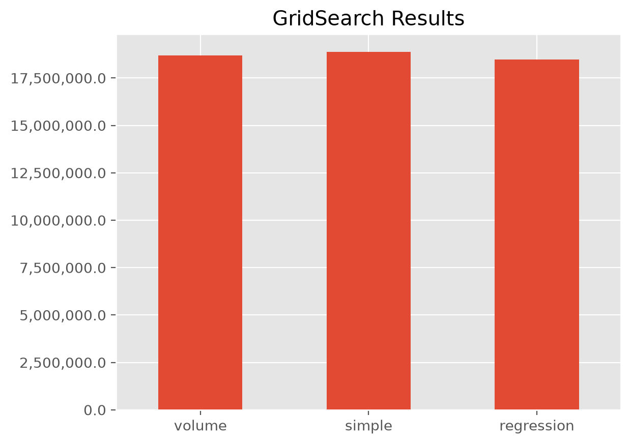
../_images/6e845bce198bcbc45cbe2cb74f78d188f57abcf9f85a8152b05a12f33488fb36.png

A couple points on the example.

The syntax for GridSearch is a near replica of scikit-learn’s GridsearchCV
The param_grid is a dictionary of hyperparamter names and possible options you may want to use.
Multiple different hyperparameters can be specified in a param_grid. Doing so will create a cartesian product of all possible assumptions.
When using a Pipeline in a GridSearch it is entirely possible that the param_grid hyperparameter names used in different steps of a the Pipeline can clash. The notation to disambiguate the hyperparameters is to specify both the step and the hyperparameter name in this fashion: step__hyperparameter

Note

All of this can be done with loops, but GridSearch provides a nice shorthand for accomplishing the same as well as parallelism when your CPU has multiple cores.

Your scoring function can be any property derived off of the fitted etimator. If capturing multiple properties is desired, multiple scoring functions can be created and stored in a dictionary.

Here we capture multiple properties of the TailBondy estimator using the GridSearch routine to test the sensitivity of the model to changing hyperparameters.

# Fit basic development to a triangle
tri = cl.load_sample('tail_sample')['paid']
dev = cl.Development(average='simple').fit_transform(tri)

# Return both the tail factor and the Bondy exponent in the scoring function
scoring = {
    'Tail Factor (tail_)': lambda x: x.tail_.values[0,0],
    'Bondy Exponent (b_)': lambda x : x.b_.values[0,0]}

# Vary the 'earliest_age' assumption in GridSearch
param_grid=dict(earliest_age=list(range(12, 120, 12)))
grid = cl.GridSearch(
    estimator=cl.TailBondy(), 
    param_grid=param_grid, 
    scoring=scoring)

grid.fit(dev).results_

	earliest_age	Tail Factor (tail_)	Bondy Exponent (b_)
0	12	1.027763	0.624614
1	24	1.027983	0.625014
2	36	1.029856	0.629534
3	48	1.037931	0.651859
4	60	1.048890	0.683528
5	72	1.046617	0.674587
6	84	1.059931	0.714418
7	96	1.072279	0.746943
8	108	1.023925	0.500000

Using GridSearch for scenario testing is entirely optional. You can write your own looping mechanisms to achieve the same result. For example:

CapeCod Sensitivity

hard

CapeCod Apriori Sensitivity

It is also possible to treat estimators themselves as hyperparameters. A GridSearch can search over Chainladder and CapeCod or any other estimator. To achieve this, you can take your param_grid dictionary and make it a list of dictionaries.

clrd = cl.load_sample('clrd')[['CumPaidLoss', 'EarnedPremDIR']].groupby('LOB').sum().loc['medmal']

grid = cl.GridSearch(
    estimator = cl.Pipeline(steps=[
        ('dev', None),
        ('model', None)]),
    param_grid = [
        {'dev': [cl.Development()],
         'dev__n_periods': [-1, 3, 7],
         'model': [cl.Chainladder()]},
        {'dev': [cl.Development()],
         'dev__n_periods': [-1, 3, 7],
         'model': [cl.CapeCod()],
         'model__decay': [0, .5, 1]}],
    scoring=lambda x : x.named_steps.model.ibnr_.sum('origin')
)

grid.fit(
    X=clrd['CumPaidLoss'], 
    sample_weight=clrd['EarnedPremDIR'].latest_diagonal)

grid.results_

	dev	dev__n_periods	model	score	model__decay
0	Development(n_periods=7)	-1	Chainladder()	1.330331e+06	NaN
1	Development(n_periods=7)	3	Chainladder()	1.254405e+06	NaN
2	Development(n_periods=7)	7	Chainladder()	1.321097e+06	NaN
3	Development(n_periods=7)	-1	CapeCod()	1.330331e+06	0.0
4	Development(n_periods=7)	-1	CapeCod()	1.278456e+06	0.5
5	Development(n_periods=7)	-1	CapeCod()	1.066857e+06	1.0
6	Development(n_periods=7)	3	CapeCod()	1.254405e+06	0.0
7	Development(n_periods=7)	3	CapeCod()	1.225866e+06	0.5
8	Development(n_periods=7)	3	CapeCod()	1.040709e+06	1.0
9	Development(n_periods=7)	7	CapeCod()	1.321097e+06	0.0
10	Development(n_periods=7)	7	CapeCod()	1.276399e+06	0.5
11	Development(n_periods=7)	7	CapeCod()	1.066171e+06	1.0

The workflow estimators are incredibly flexible for composing any compound reserving workflow into a single estimator. These succintly capture all “assumptions” and model definitions in one place.

Workflow

Contents

Workflow#

Pipeline#

VotingChainladder#

GridSearch#