Tail Estimators

Unobserved loss experience beyond the edge of a Triangle can be substantial and is a necessary part of an actuary’s analysis. This is particularly so for long tailed lines more common in commercial insurance or excess layers of loss.

With all tail estimation, we are extrapolating beyond the known data which comes with its own challenges. It tends to be more difficult to validate assumptions when performing tail estimation. Additionally, many of the techniques carry a high degree of sensitivity to the assumptions you will choose when conducting analysis.

Nevertheless, it is a necessary part of the actuary’s toolkit in estimating reserve liabilities.

Show code cell source

Hide code cell source

import chainladder as cl
import pandas as pd
import numpy as np
import matplotlib.pyplot as plt
plt.style.use('ggplot')
%config InlineBackend.figure_format = 'retina'

Basics and Commonalities

As with the Development family of estimators, the Tail module provides a variety of tail transformers that allow for the extrapolation of development patterns beyond the end of the triangle. Being transformers, we can expect that each estimator has a fit and a transform method. It is also expected that the transform method will give us back our Triangle with additional estimated parameters for incorporating our tail review in our IBNR estimates.

Tail

Every tail estimator produced a tail_ attribute which represents the point estimate of the tail of the Triangle.

Tip

Recall that the trailing underscore_ implies that these parameters are only available once we’ve fit our estimator.

We will demonstrate this property using the TailConstant estimator which we explore further below.

triangle = cl.load_sample('genins')
tail = cl.TailConstant(1.10).fit_transform(triangle)
tail.tail_

	120-Ult
(All)	1.1

Run Off

In addition to point estimates, tail estimators support run-off analysis. The ldf_ and cdf_ attribute splits the tail point estimate into enough development patterns to allow for tail run-off to be examined for at least another valuation year by default. For an annual development_grain grain, the development pattterns include two additional patterns.

tail.cdf_

	12-Ult	24-Ult	36-Ult	48-Ult	60-Ult	72-Ult	84-Ult	96-Ult	108-Ult	120-Ult	132-Ult
(All)	15.8912	4.5526	2.6054	1.7877	1.5229	1.3797	1.2701	1.2052	1.1195	1.1000	1.0514

Note

When fitting a tail estimator without first specifying a Development estimator first, chainladder assumes a volume-weighted Development. To override this, you should declare transform your triangle with a development transformer first.

For quarterly grain, there are five additional development patterns and for monthly there are thirteen.

triangle = cl.load_sample('quarterly')['paid']
tail = cl.TailCurve().fit(triangle)
# Slice just the tail entries
tail.cdf_[~tail.ldf_.development.isin(triangle.link_ratio.development)]

/home/docs/checkouts/readthedocs.org/user_builds/chainladder-python/envs/experimental/lib/python3.11/site-packages/chainladder/core/base.py:403: UserWarning: Could not infer format, so each element will be parsed individually, falling back to `dateutil`. To ensure parsing is consistent and as-expected, please specify a format.
  datetime_mapping = dict(zip(datetime_arg, pd.to_datetime(**date_inference)))

	135-Ult	138-Ult	141-Ult	144-Ult	147-Ult
(All)	1.0006	1.0005	1.0004	1.0004	1.0003

Note

The point estimate tail_ of the tail is the CDF for 135-Ult. The remaining CDFs simply represent the run-off of this tail as specified by the Tail estimator in use.

Attachment Age

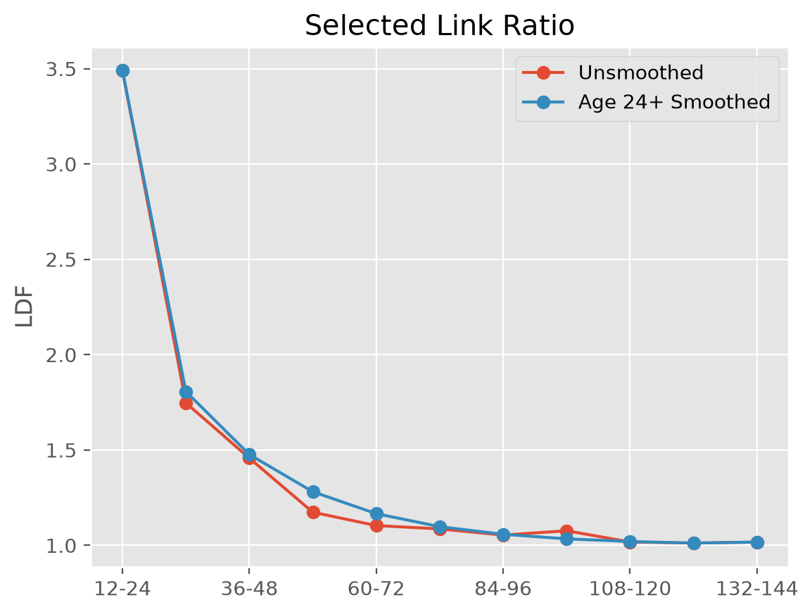
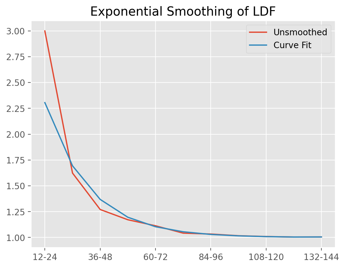
By default, tail estimators attach to the oldest development age of the Triangle. In practice, the last several known development factors of a Triangle can be unreliable and attaching the tail earlier and using it as a smoothing mechanism is preferred. All tail estimators have an attachment_age parameter that allows you to select the development age to which the tail will attach.

triangle = cl.load_sample('genins')
unsmoothed = cl.TailCurve().fit(triangle).ldf_
smoothed = cl.TailCurve(attachment_age=24).fit(triangle).ldf_

In this way, we can smooth over any volatile development patterns.

Show code cell source

Hide code cell source

pd.concat((
    unsmoothed.T.iloc[:, 0].rename('Unsmoothed'),
    smoothed.T.iloc[:, 0].rename('Age 24+ Smoothed')),
    axis=1).plot(marker='o', title='Selected Link Ratio', ylabel='LDF');

Projection period

Regardless of where you attach a tail, there will be incremental patterns to at least one year past the end of the Triangle to support run-off analysis.

This accommodates views of run-off for the oldest origin periods in your triangle for at least another year. As actuarial reviews typically occur no less than annually, this should be sufficient for examining run-off performance between actuarial valuations.

Cases arise where modeling run-off on a longer time horizon is desired. For these cases, it is possible to modify the projection_period (in months) of all Tail Esimtators by specifying the number of months you wish to extend your patterns.

# Extend tail run-off 4 years past end of Triangle.
tail = cl.TailCurve(projection_period=12*4).fit(triangle)
tail.ldf_[~tail.ldf_.development.isin(triangle.link_ratio.development)]

	120-132	132-144	144-156	156-168	168-180
(All)	1.0119	1.0071	1.0042	1.0025	1.0036

In this example, we see a higher development pattern for the last period than the ones prior. This is because the true tail run-off exceeds four years. To be clear, the projection_period has no effect on the actual estimated tail, it simply provides a longer time horizon for measuring run-off.

TailConstant

TailConstant allows you to input a tail factor as a constant. This is useful when relying on tail selections from an external source like industry data.

The tail factor supplied applies to all individual triangles contained within the Triangle object. If this is not the desired outcome, slicing individual triangles and applying TailConstant separately to each can be done.

Decay

For run-off analysis, you can control the decay of your tail. An exponential decay parameter is also available to facilitate the run off analysis described above.

tail = cl.TailConstant(tail=1.05, decay=0.95).fit_transform(triangle)
tail.ldf_

	12-24	24-36	36-48	48-60	60-72	72-84	84-96	96-108	108-120	120-132	132-144
(All)	3.4906	1.7473	1.4574	1.1739	1.1038	1.0863	1.0539	1.0766	1.0177	1.0024	1.0474

As we can see in the example, the 5% tail in the example is split between the amount to run-off over the subsequent calendar period 132-144, and the remainder, 144-Ult. The split is controlled by the decay parameter. We can always reference our tail_ point estimate.

tail.tail_

	120-Ult
(All)	1.05

Examples

[DevelopmentConstant Callable]

hard

DevelopmentConstant Callable

TailCurve

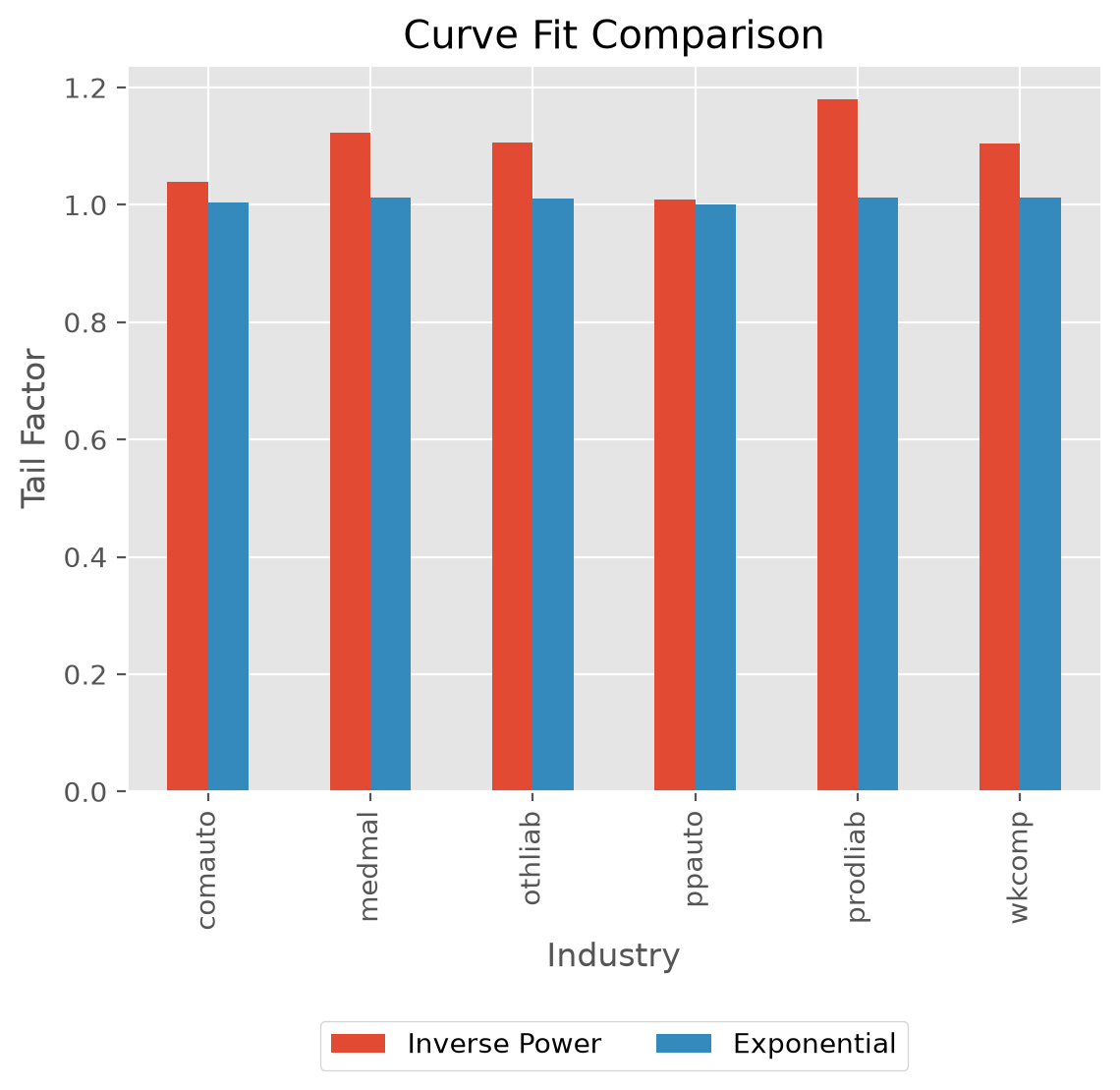
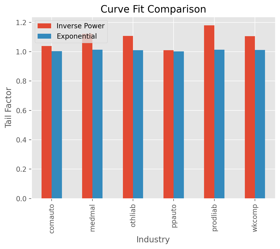
TailCurve allows for extrapolating a tail factor using curve fitting. Currently, exponential decay of LDFs and inverse power curve are supported.

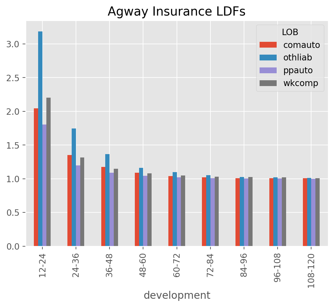
clrd = cl.load_sample('clrd').groupby('LOB').sum()['CumPaidLoss']
cdf_ip = cl.TailCurve(curve='inverse_power').fit(clrd).tail_
cdf_xp = cl.TailCurve(curve='exponential').fit(clrd).tail_

Show code cell source

Hide code cell source

ax = pd.concat((cdf_ip.rename("Inverse Power"),
           cdf_xp.rename("Exponential")), axis=1).plot(
        kind='bar', title='Curve Fit Comparison',
        xlabel='Industry', ylabel='Tail Factor')

ax.legend(loc='center', bbox_to_anchor=(.5, -.35), facecolor='white', ncol=2);

Regression parameters

Underlying the curve fit is an OLS regression which generates both a slope_ and intercept_ term.

For the exponential curve fit with slope, \(\beta\) and intercept \(\alpha\), the tail factor is:

(1)\[ \prod_{i}^{N}1+exp(\beta X+\alpha ) \]

For the inverse_power curve, the tail factor is:

(2)\[ \prod_{i}^{N}1+exp(\alpha) X^{\beta} \]

Where \(X\) is your selected link ratios and \(N\) is the number of years you wish to extrapolate the tail_

Deriving the tail_ factor manually:

triangle = cl.load_sample('genins')
tail = cl.TailCurve('exponential').fit(triangle)
tail.tail_

	120-Ult
(All)	1.029499

A manual calculation using (1) above:

np.prod(
    (1+np.exp(
        np.arange(triangle.shape[-1],
                  triangle.shape[-1] + tail.extrap_periods) * 
        tail.slope_.values + tail.intercept_.values)
    )
)

np.float64(1.0294991710529175)

For completeness, let’s also confirm (2):

tail = cl.TailCurve('inverse_power').fit(triangle)
tail.tail_

	120-Ult
(All)	1.29243

np.prod(
    1 + np.exp(tail.intercept_.values) * 
    (
        np.arange(
            triangle.shape[-1], 
            triangle.shape[-1] + tail.extrap_periods
        ) ** tail.slope_.values)
)

np.float64(1.292430311543694)

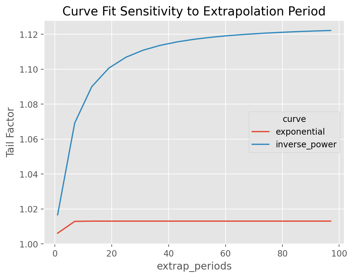
Extrapolation Period

From these formulas, the actuary has control over the parameter, \(N\) which represents how far out how far beyond the edge of Results for the inverse_power curve are sensitive to this parameter as it tends to converge slowly to its asymptotic value. This parameter can be controlled using the extrap_periods hyperparamter.

Tip

Exponential decay is generally rapid and is less sensitive to the extrap_period argument than the inverse power fit.

Show code cell source

Hide code cell source

tri = cl.load_sample('clrd').groupby('LOB').sum().loc['medmal', 'CumPaidLoss']

# Create a function to grab the scalar tail value.
def scoring(model):
    """ Scoring functions must return a scalar """
    return model.tail_.iloc[0, 0]

# Create a grid of scenarios
param_grid = dict(
    extrap_periods=list(range(1, 100, 6)),
    curve=['inverse_power', 'exponential'])

# Fit Grid
model = cl.GridSearch(cl.TailCurve(), param_grid=param_grid, scoring=scoring).fit(tri)

# Plot results
model.results_.pivot(columns='curve', index='extrap_periods', values='score').plot(
    grid=True, ylim=(1,None), title='Curve Fit Sensitivity to Extrapolation Period').set(
    ylabel='Tail Factor');

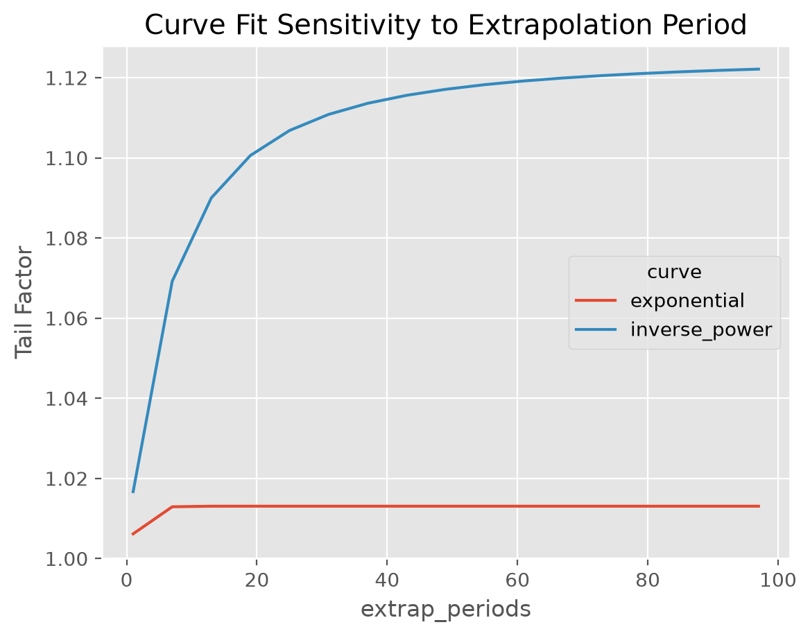
This example demonstrates the extrap_periods functionality of the TailCurve estimator. The estimator defaults to extrapolating out 100 periods. However, we can see that the “Inverse Power” curve fit doesn’t converge to its asymptotic value even with 100 periods whereas the “exponential” converges within 10 periods.

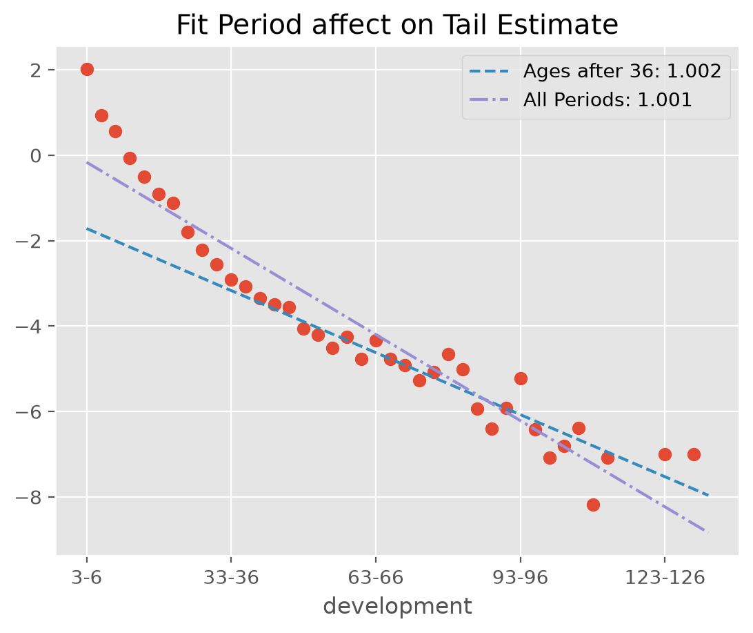
Fit period

The default behavior of TailCurve is to include all cdf_ patterns from the Triangle in extrapolating the tail. Often, the data assumptions of linearity will be violated when using all selected patterns. In those cases, you can use fit_period=(start_age, end_age) for fitting to a contiguous set of patterns.

dev = cl.Development().fit_transform(cl.load_sample('quarterly')['paid'])
fit_all = cl.TailCurve().fit(dev)
exclude = cl.TailCurve(fit_period=(36, None)).fit(dev)

/home/docs/checkouts/readthedocs.org/user_builds/chainladder-python/envs/experimental/lib/python3.11/site-packages/chainladder/core/base.py:403: UserWarning: Could not infer format, so each element will be parsed individually, falling back to `dateutil`. To ensure parsing is consistent and as-expected, please specify a format.
  datetime_mapping = dict(zip(datetime_arg, pd.to_datetime(**date_inference)))

Show code cell source

Hide code cell source

obs = (dev.ldf_ - 1).T.iloc[:, 0]
obs[obs < 0] = np.nan

ax = np.log(obs).rename('Selected LDF').plot(
    style=' ', marker='o', title=f'Fit Period affect on Tail Estimate');
pd.Series(
    np.arange(1, dev.ldf_.shape[-1] + 1) * exclude.slope_.sum().values + exclude.intercept_.sum().values, 
    index=dev.ldf_.development, 
    name=f'Ages after 36: {round(exclude.tail_.values[0,0], 3)}').plot(
    ax=ax, style = '--', legend=True);
pd.Series(
    np.arange(1, dev.ldf_.shape[-1] + 1) * fit_all.slope_.sum().values + fit_all.intercept_.sum().values, 
    index=dev.ldf_.development, 
    name=f'All Periods: {round(fit_all.tail_.values[0,0], 3)}').plot(
    ax=ax, style = '-.', legend=True);

Warning

The nature of curve fitting with log and exp transforms is inappropriate for development factors less than 1.0. The default behavior of TailCurve is to ignore these observations when determining the OLS regression parameters. You can force errors by setting the errors argument to “raise”.

dev = cl.TailCurve(errors='raise')
# This will fail because of LDFs < 1 and our choice to 'raise' errors
dev.fit(cl.load_sample('quarterly')['paid'])

You can also use a list to of booleans to specify which values you want to include. This allows for finer grain control over excluding outliers from your analysis. The following two estimators are equivalent.

(cl.TailCurve(fit_period=[False] * 11 + [True] * 33).fit(dev).cdf_ ==
 cl.TailCurve(fit_period=(36, None)).fit(dev).cdf_)

np.True_

Examples

[Attachment Age Smoothing]

easy

Attachment Age Smoothing

[TailCurve Extrapolation]

medium

Extrapolation Period Sensitivity

[TailCurve Basics]

easy

TailCurve Basics

[Party, 2013]

TailBondy

Most people are familiar with the Bondy tail know it as a basic method that assumes the tail_ is just a repeat of the last available ldf_.

Indeed, without any hyperparameter selection, this is how TailBondy works.

triangle = cl.load_sample('genins')
dev = cl.Development().fit_transform(triangle)
dev.ldf_.iloc[..., -1]

	108-120
(All)	1.0177

tail = cl.TailBondy().fit(triangle)
tail.tail_

	120-Ult
(All)	1.017725

This simple relationship has a more generalized form. If we define the ldf_ at time \(n\) as \(f(n-1)\) and assume that \(f(n) = f(n-1)^{B}\), it follows that the tail \(F(n)\) can be defined as:

(3)\[ F(n)=f(n-1)^{B}f(n-1)^{B^{2}}...=f(n-1)^{\frac{B}{1-B}} \]

where \(B\) is some constant, and if \(B\) is \(\frac{1}{2}\), then we obtain Bondy’s original tail formulation.

Rather than using the only the last known development factor or setting \(B=\frac{1}{2}\), we can stablize things using more ldf_ using the earliest_age parameter. We can then minimize the difference in the the assumed relationship \(f(n) = f(n-1)^{B}\) and our data to estimate \(B\).

This is often refered to as the Generalized Bondy method.

triangle = cl.load_sample('tail_sample')['paid']
dev = cl.Development(average='simple').fit_transform(triangle)

# Estimate the Bondy Tail
tail = cl.TailBondy(earliest_age=12).fit(dev)
tail.tail_

	120-Ult
(All)	1.027763

Using our formulation (3) above, we can manually estimate our tail using our earliest ldf_ and our Bondy constant b_.

# Get last fitted LDF of the model
last_fitted_ldf = (tail.earliest_ldf_ ** (tail.b_ ** 8))

# Calculate the tail using the Bondy formula above
last_fitted_ldf ** (tail.b_ / (1-tail.b_))

	paid
Total
Total	1.027756

[Party, 2013]

TailClark

TailClark is a continuation of the ClarkLDF model. Familiarity with ClarkLDF will aid in understanding this Estimator. The growth curve approach used by Clark produces development patterns for any age including ages beyond the edge of the Triangle.

An example completing Clark’s model:

genins = cl.load_sample('genins')
dev = cl.ClarkLDF()
tail = cl.TailClark()
tail.fit(dev.fit_transform(genins)).ldf_

	12-24	24-36	36-48	48-60	60-72	72-84	84-96	96-108	108-120	120-132	132-144
(All)	4.0951	1.7205	1.3424	1.2005	1.1306	1.0910	1.0665	1.0504	1.0393	1.0313	1.2540

Coupled with attachment_age one could use any Development estimator and replicate the ClarkLDF estimator.

genins = cl.load_sample('genins')
tail = cl.TailClark(attachment_age=12)
tail.fit(cl.Development().fit_transform(genins)).ldf_

	12-24	24-36	36-48	48-60	60-72	72-84	84-96	96-108	108-120	120-132	132-144
(All)	4.0951	1.7205	1.3424	1.2005	1.1306	1.0910	1.0665	1.0504	1.0393	1.0313	1.2540

Truncated patterns

Clark warns of the dangers of extrapolating too far beyond the edge of a Triangle, particularly with a heavy tailed distribution. In these cases, it is suggested that a suitable cut-off age or truncation_age be established where losses are considered fully developed. This is very similar to the extrap_periods parameter of TailCurve, however, it is expressed as an age (in months) as opposed to a period length.

tail = cl.TailClark(truncation_age=245)
tail.fit(dev.fit_transform(genins)).cdf_

	12-Ult	24-Ult	36-Ult	48-Ult	60-Ult	72-Ult	84-Ult	96-Ult	108-Ult	120-Ult	132-Ult
(All)	19.2089	4.6907	2.7264	2.0309	1.6917	1.4963	1.3715	1.2860	1.2243	1.1780	1.1423

[Clark, 2003]