Data Adjustments#
There are many useful data adjustments in reserving that are not necessarily direct
IBNR models nor development factor selections. This module covers those implemented
by chainladder. In all cases, these adjustments are most useful when used
as part of a larger workflow.
BootstrapODPSample#
Simulations#
:class:BootstrapODPSample is a transformer that simulates new triangles
according to the ODP Bootstrap model. That is both the index and column
of the Triangle must be of unity length. Upon fitting the Estimator, the
index will contain the individual simulations.
import chainladder as cl
import pandas as pd

raa = cl.load_sample('raa')
cl.BootstrapODPSample(n_sims=500).fit_transform(raa)
/home/docs/checkouts/readthedocs.org/user_builds/chainladder-python/envs/experimental/lib/python3.11/site-packages/chainladder/adjustments/bootstrap.py:311: UserWarning: 'where' used without 'out', expect unitialized memory in output. If this is intentional, use out=None.
  hat = xp.diagonal(xp.sqrt(xp.divide(1, abs(1 - hat), where=(1 - hat) != 0)))
| Triangle Summary | |
|---|---|
| Valuation: | 1990-12 |
| Grain: | OYDY |
| Shape: | (500, 1, 10, 10) |
| Index: | [Simulation_#] |
| Columns: | [values] |
Note
The BootstrapODPSample can only apply to single triangles as it needs the
index axis to be free to hold the different triangle simluations.
Dropping#
The Estimator has full dropping support consistent with the Development estimator.
This allows for eliminating problematic values from the sampled residuals.
cl.BootstrapODPSample(n_sims=100, drop=[('1982', 12)]).fit_transform(raa)
/home/docs/checkouts/readthedocs.org/user_builds/chainladder-python/envs/experimental/lib/python3.11/site-packages/chainladder/adjustments/bootstrap.py:311: UserWarning: 'where' used without 'out', expect unitialized memory in output. If this is intentional, use out=None.
  hat = xp.diagonal(xp.sqrt(xp.divide(1, abs(1 - hat), where=(1 - hat) != 0)))
| Triangle Summary | |
|---|---|
| Valuation: | 1990-12 |
| Grain: | OYDY |
| Shape: | (100, 1, 10, 10) |
| Index: | [Simulation_#] |
| Columns: | [values] |
Deterministic methods#
The class only simulates new triangles from which you can generate statistics about parameter and process uncertainty. This allows for converting the various deterministic IBNR methods into stochastic methods.
Like the Development estimators, The BootstrapODPSample allows for ommission
of certain residuals from its sampling algorithm with a suite of “dropping”
parameters. See :ref:Omitting Link Ratios<dropping>.
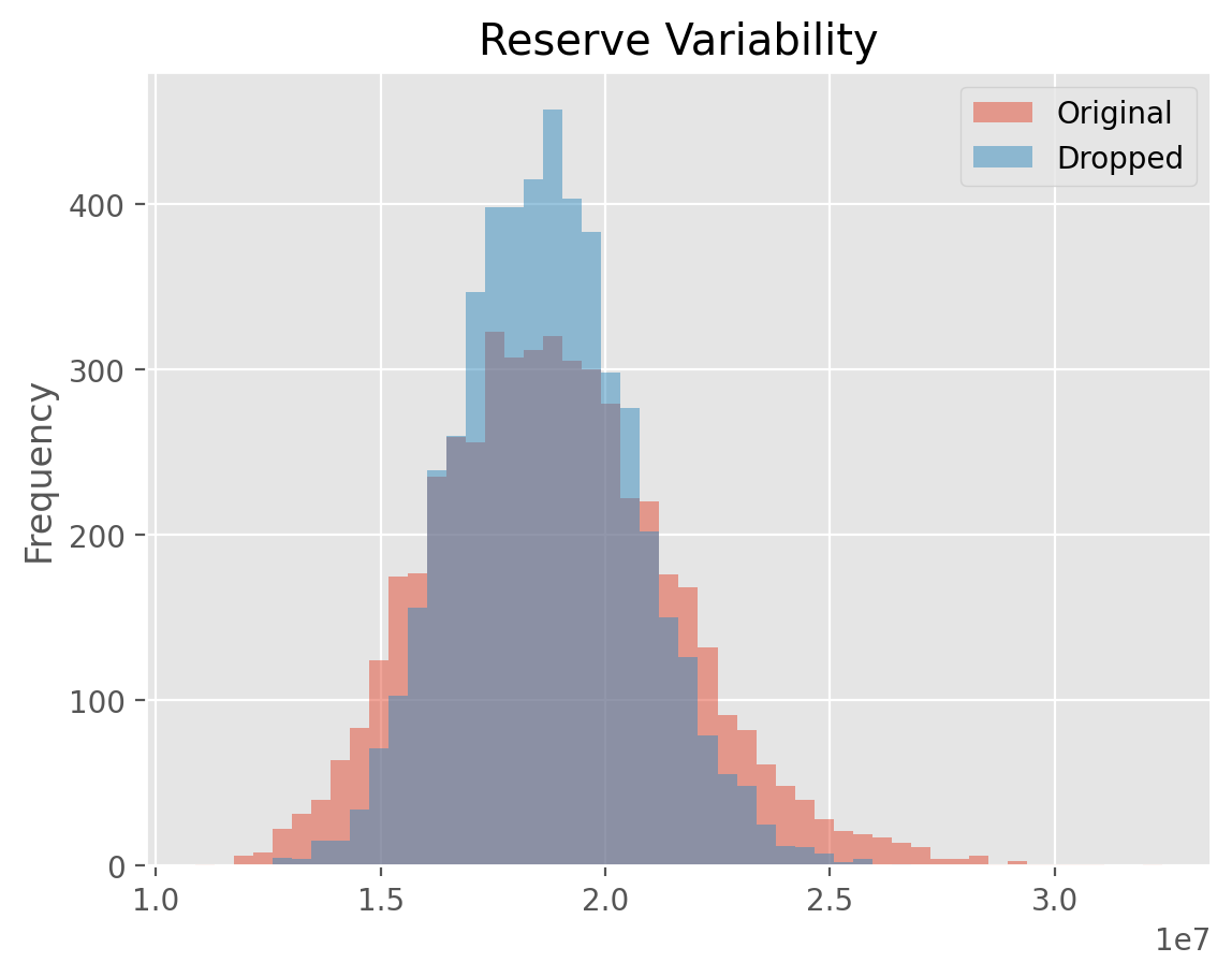
Examples#
[BootstrapODPSample Variability]
BerquistSherman#
:class:BerquistSherman provides a mechanism of restating the inner diagonals of a
triangle for changes in claims practices. These adjustments can materialize in
case incurred and paid amounts as well as closed claims count development.
In all cases, the adjustments retain the unadjusted latest diagonal of the
triangle. For the Incurred adjustment, an assumption of the trend rate in
average open case reserves must be supplied. For the adjustments to paid
amounts and closed claim counts, an estimator, such as Chainladder is needed
to calulate ultimate reported count so that the disposal_rate_ of the
model can be calculated.
Adjustments#
The BerquistSherman technique requires values for paid_amount, incurred_amount,
reported_count, and closed_count to be available in your Triangle. Without
these triangles, the BerquistSherman model cannot be used. If these conditions
are satisfied, the BerquistSherman technique adjusts all triangles except the
reported_count triangle.
The Estimator wraps all adjustments up in its adjusted_triangle_ property.
triangle = cl.load_sample('berqsherm').loc['MedMal']
berq = cl.BerquistSherman(
    paid_amount='Paid', incurred_amount='Incurred',
    reported_count='Reported', closed_count='Closed',
    trend=0.15).fit(triangle)

# Only Reported triangle is left unadjusted
(triangle / berq.adjusted_triangle_)['Reported']
| 12 | 24 | 36 | 48 | 60 | 72 | 84 | 96 | |
|---|---|---|---|---|---|---|---|---|
| 1969 | 1.0000 | 1.0000 | 1.0000 | 1.0000 | 1.0000 | 1.0000 | 1.0000 | 1.0000 |
| 1970 | 1.0000 | 1.0000 | 1.0000 | 1.0000 | 1.0000 | 1.0000 | 1.0000 | |
| 1971 | 1.0000 | 1.0000 | 1.0000 | 1.0000 | 1.0000 | 1.0000 | ||
| 1972 | 1.0000 | 1.0000 | 1.0000 | 1.0000 | 1.0000 | |||
| 1973 | 1.0000 | 1.0000 | 1.0000 | 1.0000 | ||||
| 1974 | 1.0000 | 1.0000 | 1.0000 | |||||
| 1975 | 1.0000 | 1.0000 | ||||||
| 1976 | 1.0000 |
Latest Diagonal#
Only the inner diagonals of the Triangle are adjusted. This allows the
adjusted_triangle_ to be a drop in surrogate for the original.
(triangle / berq.adjusted_triangle_)['Paid']
| 12 | 24 | 36 | 48 | 60 | 72 | 84 | 96 | |
|---|---|---|---|---|---|---|---|---|
| 1969 | 2.0714 | 3.3635 | 1.5968 | 1.3856 | 0.7545 | 1.2105 | 0.8862 | 1.0000 |
| 1970 | 0.7603 | 2.2084 | 1.2420 | 0.9964 | 0.8729 | 1.4994 | 1.0000 | |
| 1971 | 1.7663 | 4.3464 | 1.7429 | 1.2899 | 0.7629 | 1.0000 | ||
| 1972 | 0.7129 | 2.3514 | 1.6228 | 1.2540 | 1.0000 | |||
| 1973 | 1.3234 | 1.6029 | 0.7186 | 1.0000 | ||||
| 1974 | 1.4519 | 2.8518 | 1.0000 | |||||
| 1975 | 1.3604 | 1.0000 | ||||||
| 1976 | 1.0000 |
Transform#
BerquistSherman is strictly a data adjustment to the Triangle and it does
not attempt to estimate development patterns, tails, or ultimate values. Once
transform is invoked on a Triangle, the adjusted_triangle_ takes the
place of the existing Triangle.
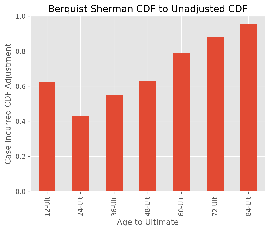
Examples#
[BerquistSherman Adjustment]
ParallelogramOLF#
The :class:ParallelogramOLF estimator is used to on-level a Triangle using
the parallogram technique. It requires a “rate history” and supports both
vertical line estimates as well as the more common effective date estimates.
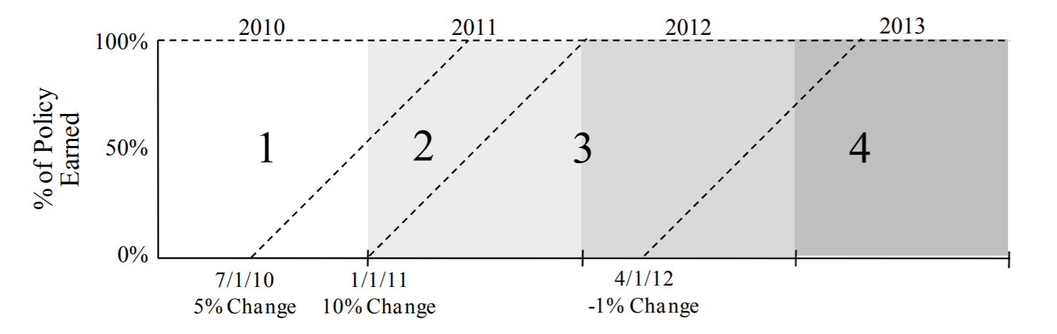
Rate History#
The Estimator requires a rate history that has, at a minimum, the rate changes and date-like columns reflecting the corresponding effective dates of the rate changes.
rate_history = pd.DataFrame({
    'EffDate': ['2016-07-15', '2017-03-01', '2018-01-01', '2019-10-31'],
    'RateChange': [0.02, 0.05, -.03, 0.1]})
rate_history
| EffDate | RateChange | |
|---|---|---|
| 0 | 2016-07-15 | 0.02 |
| 1 | 2017-03-01 | 0.05 |
| 2 | 2018-01-01 | -0.03 |
| 3 | 2019-10-31 | 0.10 |
The ParallelogramOLF maps the rate history using the change_col and date_col
arguments. Once mapped, the transformer provides an olf_ property
representing the on-level factors from the parallelogram on-leveling technique.
When used as a transformer, it retains your Triangle as it is, but then adds
the olf_ property to your Triangle.
data = pd.DataFrame({
    'Year': [2016, 2017, 2018, 2019, 2020],
    'EarnedPremium': [10_000]*5})
prem_tri = cl.Triangle(data, origin='Year', columns='EarnedPremium', cumulative = True)
prem_tri = cl.ParallelogramOLF(rate_history, change_col='RateChange', date_col='EffDate').fit_transform(prem_tri)
prem_tri.olf_
| 2020 | |
|---|---|
| 2016 | 1.0185 |
| 2017 | 1.0011 |
| 2018 | 0.9854 |
| 2019 | 1.0000 |
| 2020 | 1.0000 |
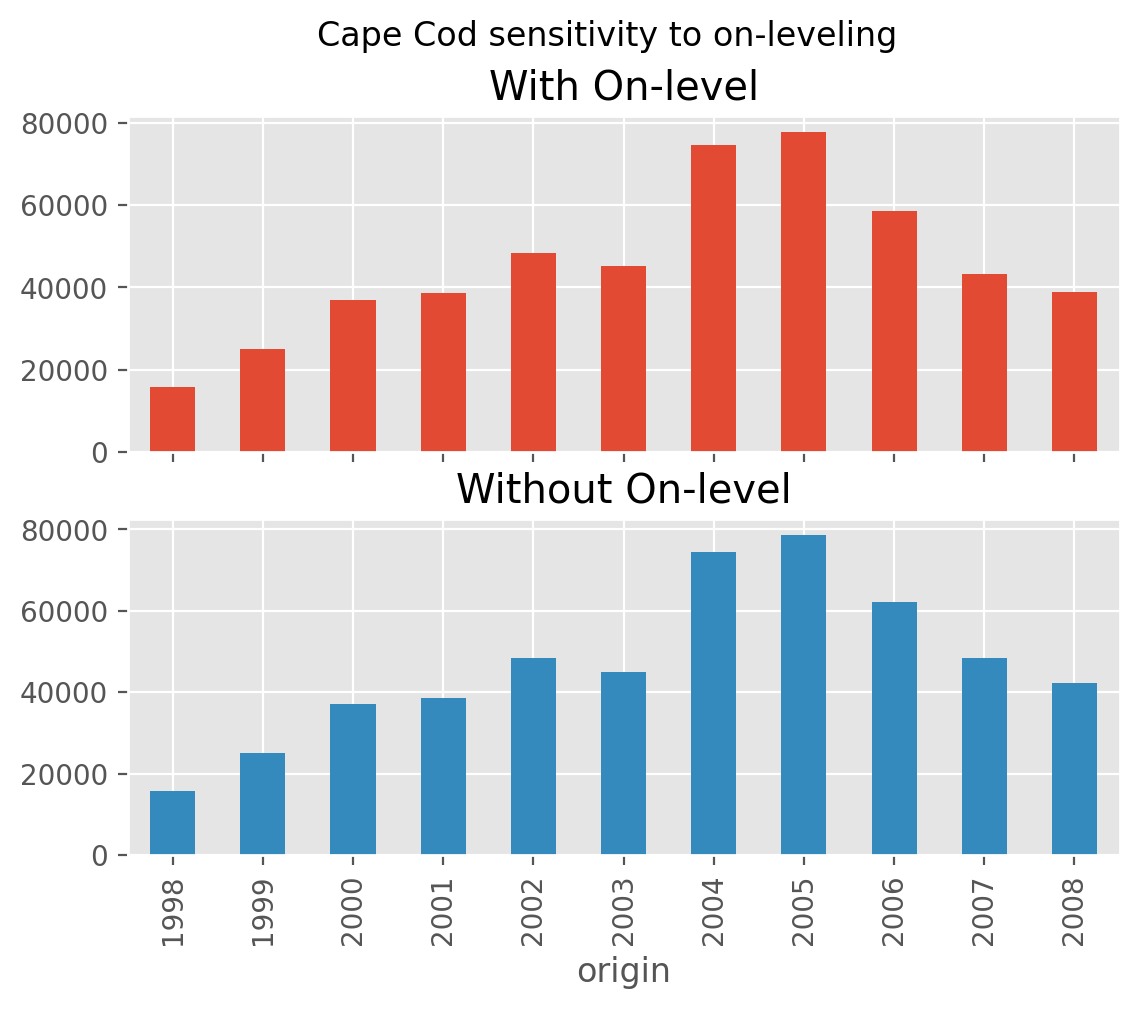
Input to CapeCod#
This estimator can be used within other estimators that depend on on-leveling,
such as the :class:CapeCod method. This is accomplished by passing a
ParallelogramOLF transformed Triangle to the CapeCod estimator.
Examples#
[CapeCod Onleveling]
Trend#
The :class:Trend estimator is a convenience estimator that allows for compound
trends to be used in other estimators that have a trend assumption. This
enables more complex trend assumptions to be used.
ppauto_loss = cl.load_sample('clrd').groupby('LOB').sum().loc['ppauto', 'CumPaidLoss']
ppauto_prem = cl.load_sample('clrd').groupby('LOB').sum() \
                .loc['ppauto']['EarnedPremDIR'].latest_diagonal

# Simple trend
a = cl.CapeCod(trend=0.05).fit(ppauto_loss, sample_weight=ppauto_prem).ultimate_.sum()

# Equivalent using a Trend Estimator. This allows us to convert to more complex trends
b = cl.CapeCod().fit(cl.Trend(.05).fit_transform(ppauto_loss), sample_weight=ppauto_prem).ultimate_.sum()
a == b
np.True_
Multipart Trend#
A multipart trend can be achieved if passing a list of trends and corresponding
dates. Dates should be represented as a list of tuples (start, end).
The default start and end dates for a Triangle are its valuation_date and
its earliest origin date.
ppauto_loss = cl.load_sample('clrd').groupby('LOB').sum().loc['ppauto', 'CumPaidLoss']
cl.Trend(
    trends=[.05, .03],
    dates=[('1997-12-31', '1995-01-01'),('1995-01-01', '1992-07-01')]
).fit(ppauto_loss).trend_.round(2)
| 12 | 24 | 36 | 48 | 60 | 72 | 84 | 96 | 108 | 120 | |
|---|---|---|---|---|---|---|---|---|---|---|
| 1988 | 1.2400 | 1.2400 | 1.2400 | 1.2400 | 1.2400 | 1.2400 | 1.2400 | 1.2400 | 1.2400 | 1.2400 |
| 1989 | 1.2400 | 1.2400 | 1.2400 | 1.2400 | 1.2400 | 1.2400 | 1.2400 | 1.2400 | 1.2400 | |
| 1990 | 1.2400 | 1.2400 | 1.2400 | 1.2400 | 1.2400 | 1.2400 | 1.2400 | 1.2400 | ||
| 1991 | 1.2400 | 1.2400 | 1.2400 | 1.2400 | 1.2400 | 1.2400 | 1.2400 | |||
| 1992 | 1.2300 | 1.2300 | 1.2300 | 1.2300 | 1.2300 | 1.2300 | ||||
| 1993 | 1.1900 | 1.1900 | 1.1900 | 1.1900 | 1.1900 | |||||
| 1994 | 1.1600 | 1.1600 | 1.1600 | 1.1600 | ||||||
| 1995 | 1.1000 | 1.1000 | 1.1000 | |||||||
| 1996 | 1.0500 | 1.0500 | ||||||||
| 1997 | 1.0000 |